MR9–MR12 - Normal models, standardisation and inverse probabilities
Connect a Normal probability curve with sample histograms (MR9) and locate its symmetry and inflections (MR11). Standardise and transform a Normal variable (MR10), then calculate probabilities and inverse boundaries, including unknown parameters (MR12).
A normal curve describes probability through area
A sensor records lengths with mean 80 cm and standard deviation 6 cm. How high should its reading be before it falls in the largest 5%? The answer depends on area under a probability curve, not on the tallest point of a sample histogram.
You already know
Variance is the square of standard deviation. A histogram uses area for frequency; scaling total area to 1 makes each bar's area an observed proportion. Samples vary, even when drawn from the same population.
Start with the model, then ask how observations from it behave.
Normal distribution
A Normal distribution is a continuous, symmetric, bell-shaped probability model. Write , where is its mean and its standard deviation. The second parameter is variance. Its line of symmetry is and its inflections, where the curve changes between concave upwards and concave downwards, are at .
Thus the sensor model is , with symmetry at 80 cm and inflections at 74 and 86 cm. Increasing spreads the same total area over a wider range and lowers the peak; changing shifts the curve's centre.
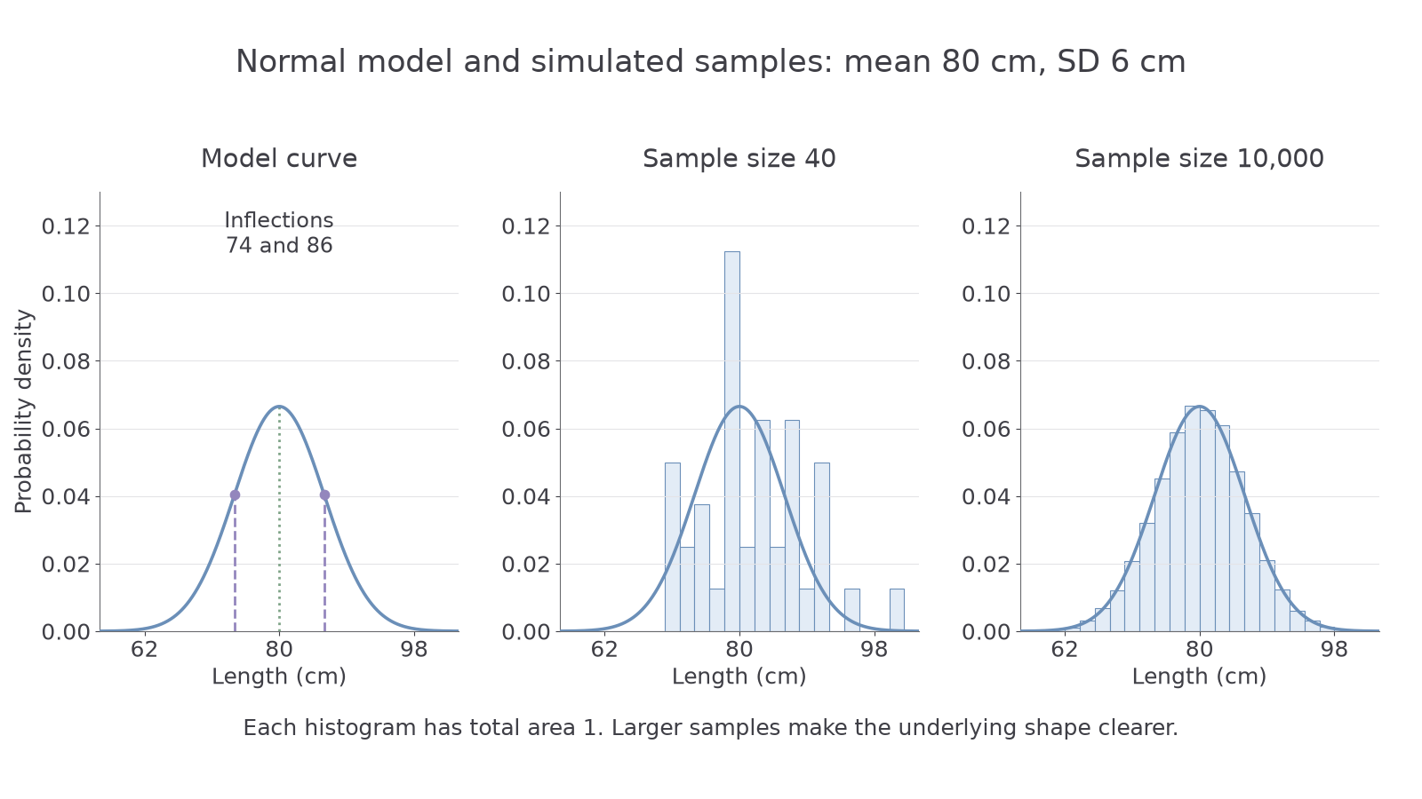
The total model area is 1, and an interval's area is its probability. Height is a density, not a probability. A surprising consequence is , even though the density is largest there. A single point has no width and hence no area; every non-empty interval around 80 has positive probability. Consequently and give the same Normal probability at a fixed boundary, unlike a discrete count.
Histograms from increasingly large samples of a Normal population tend to reveal the Normal curve. With suitable bins and area scaled to 1, the bars describe observed proportions and the curve gives model probabilities. The picture uses simulated samples, not real sensor readings: the larger sample makes the underlying shape clearer, although binning and chance variation remain.
The model's mean and variance describe the limiting values approached by statistics from increasingly large samples. A particular sample mean or sample variance need not equal them. Calculating the theoretical moments from the curve, or proving transformation results, is beyond what you need here. A symmetric-looking histogram alone also cannot guarantee a Normal population or accurate tail predictions.
Key idea
Use areas for probability and standard deviation for horizontal distance. Larger samples can make a model's shape clearer; they do not remove sampling variation or establish the model by themselves.
Separate the variance parameter from the locations of the inflections.
Convert bounds to the standard Normal scale
Standardisation measures how far a value lies above or below the mean, in standard-deviation units.
Standardisation
For ,
The sheet supplies a sample-mean expression for a later topic, but not this single-observation formula. Not in the formula sheet: learn it.
The denominator is positive, so inequalities retain their direction. Define . Normal symmetry gives . Subtracting two lower-tail areas gives the probability between their bounds.
Worked example 1: an area below a reading
Question. For , calculate , to three significant figures.
Plan. Standardise 89 using standard deviation 6, then evaluate a lower-tail probability.
Why this step? The required area is already below the bound, so no complement is needed.
Answer. The probability is 0.933, to three significant figures.
Check. The upper tail is , and the two probabilities total 1.
Change only the lower bound: instead of extending indefinitely to the left, start the region at 74. The upper bound stays 89.
Worked example 2: an interval between readings
Question. For the same model, calculate , to three significant figures.
Plan. Standardise the new lower bound, then subtract its lower-tail area.
Why this step? Removing the whole area below 74 leaves exactly the region from 74 to 89.
Answer. The probability is 0.775, to three significant figures.
Check. The excluded tails are and ; the interval and both tails total 1.
A calculator can work directly with lower bound 74, upper bound 89, mean 80 and standard deviation 6. Check its parameter convention and distinguish cumulative probability from inverse probability. For an infinite tail use its supported tail/infinity option, or a sufficiently distant finite bound whose omitted area is negligible at the stated accuracy. Retain unrounded values for subsequent calculations.
Watch out
Wrong: . Right: the variance is 36 but the standard deviation is 6, giving . A plausible calculator output does not repair the wrong model parameters.
Use the same area decisions with a new centre and spread.
A linear transformation changes centre and spread
Changing the unit or zero of a measurement transforms its centre and spread. A negative scale also reverses which readings are high and low.
Linear transformation of a Normal variable
If and , with , then
Proof is not required. Not in the formula sheet: learn it.
Continue this lesson.
You’re previewing NovaLearn without an account. Create a free account to read the rest.
Create free account