Mf8 - Building, comparing and refining function models | OCR A-Level Mathematics B (MEI)

Can you trust a function simply because it matches the measurements? Mf8 uses functions to model a practical situation, with particular care over limitations and refinements. You will build and compare predictions, interpret their assumptions, and carry a decision through a complete problem-solving cycle.

Choosing variables assumptions and a domain

A tank contains $20$ litres now and $100$ litres after $8$ minutes. Can those two measurements tell you how much water it contains at every other time? A straight line gives a quick prediction, but choosing a straight line already makes an assumption about the filling.

You already know

A linear function has a constant gradient: equal input increases give equal output increases. A function's domain states its permitted inputs; a practical model may need a narrower domain than its algebraic formula.

First specify the purpose: predict volume during filling, rather than water temperature or filling cost. Let $t$ be time in minutes after filling starts, and $V(t)$ be volume in litres. The initial volume is known; what remains to model is how it changes.

Function model

A function model is a simplified mathematical description that assigns an output to each permitted input to answer a practical question. Its variables, assumptions and useful domain belong to the model. For example, a constant-rate volume model treats time as continuous. A fractional number of parcels is not a valid input to a model of a parcel count.

An assumption simplifies the situation. Here, constant net inflow means inflow minus outflow remains constant; it does not require there to be no outflow at all.

Constant-rate model

If an output starts at $V_0$ and changes at constant rate $r$ ,

V(t)=V_0+rt

Use units consistent with $t$ and restrict the domain to where the constant-rate assumption and physical constraints apply.

Not in the formula sheet: learn it.

The formula is a structure, not evidence that a rate is constant. Fit its parameters from the measurements, then ask whether the structure is sensible.

Worked example 1: constructing a filling model

Question. A $100$ -litre tank contains $20$ litres at $t=0$ and reaches capacity at $t=8$ minutes. Construct a linear model during these eight minutes, interpret its gradient and predict the volume at $t=3$ .

Plan. Use the initial volume as intercept and the change per minute as gradient.

\begin{aligned} r&=\frac{100-20}{8-0}=10 && \text{litres gained per minute} \\ L(t)&=20+10t,\quad0\le t\le8 && \text{fit the two endpoints} \\ L(3)&=20+10(3)=50 && \text{interpolate} \end{aligned}

Why this step? A linear model assumes constant net inflow; the gradient is its physical rate, not just a number attached to $t$ .

Answer. $L(t)=20+10t$ , for $0\le t\le8$ , with a constant net inflow of $10\,\mathrm{litres\,min^{-1}}$ . It predicts $50$ litres at $3$ minutes.

Check. $L(0)=20$ and $L(8)=100$ . These checks confirm the fit, not the assumption of constant flow between the measurements.

Change only the unit of the input: describe the same filling process in seconds. The physical rate has not changed, but its numerical coefficient must.

Worked example 2: changing the time unit

Question. Write the same linear filling model using $s$ , the number of seconds after filling starts. State its useful domain and predict the volume at $s=180$ .

Plan. Convert the elapsed times to seconds before finding the new coefficient.

\begin{aligned} 8\text{ minutes}&=480\text{ seconds} && \text{convert the input unit} \\ r&=\frac{100-20}{480}=\frac16 && \text{litres gained per second} \\ W(s)&=20+\frac{s}{6},\quad0\le s\le480 && \text{state the useful domain} \\ W(180)&=20+\frac{180}{6}=50 && \text{evaluate at the new input} \end{aligned}

Why this step? A coefficient has units: $10$ litres per minute is $\tfrac16$ litre per second. Keeping the number $10$ after changing the time unit would describe a different process.

Answer. $W(s)=20+s/6$ for $0\le s\le480$ , assuming constant net inflow. It predicts $50$ litres at $180$ seconds.

Check. $W(480)=100$ , and $180$ seconds is $3$ minutes, agreeing with $L(3)=50$ .

Interpolation uses an input within the measured span; extrapolation goes beyond it. The first formula gives $L(12)=140$ , exceeding the capacity. Its algebraic domain is $\mathbb R$ , but its useful domain here is only $[0,8]$ .

Counted objects need a discrete domain. A delivery costing £ $36$ plus £ $2$ per parcel has $C(n)=36+2n$ for integers $n\ge0$ . Average cost is $C(n)/n=36/n+2$ , for integers $n\ge1$ ; averaging the cost over zero parcels is undefined.

Watch out

Wrong: “The formula accepts $t=12$ , so its prediction is valid.” Right: check the useful domain and capacity. A permissible algebraic substitution can still give an unsupported practical prediction.

Now construct a line from different measurements and say what its coefficient means physically.

Comparing predictions with fresh data

A model should earn your trust on data it was not chosen to fit.

Return to the tank that reaches capacity after $8$ minutes. Additional measurements show progressively smaller gains:

$t$ , minutes	$0$	$2$	$4$	$6$	$8$
Volume, litres	$20$	$52$	$76$	$92$	$100$
$L(t)=20+10t$	$20$	$40$	$60$	$80$	$100$

Try $Q(t)=a+bt+ct^2$ . Fitting the observations at $0,4,8$ gives

\begin{aligned} a&=20 && \text{initial measurement} \\ 4b+16c&=56 && \text{measurement at }t=4 \\ 8b+64c&=80 && \text{measurement at }t=8 \\ 32c&=-32\implies c=-1 && \text{subtract twice the second line} \\ b&=18 && \text{substitute back} \end{aligned}

Thus $Q(t)=20+18t-t^2$ . It also predicts $52$ and $92$ at the other tabulated times.

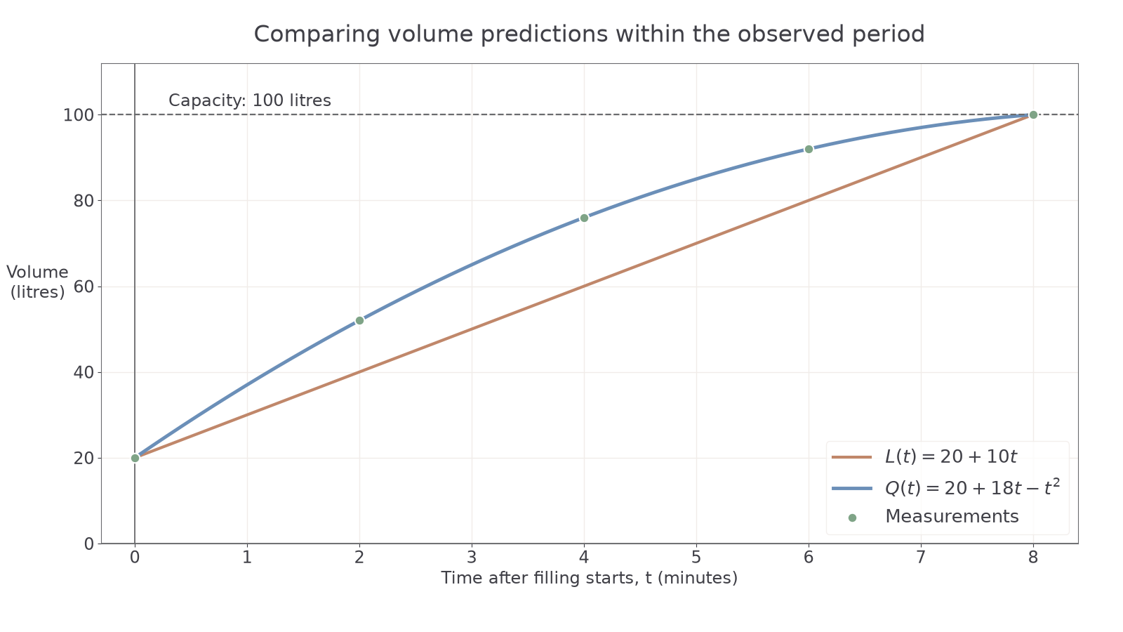
Linear and quadratic tank-volume models compared with measurements over eight minutes

There are infinitely many curves through the same two endpoints. In fact, $20+10t+kt(t-8)$ gives $20$ at $t=0$ and $100$ at $t=8$ , for every real $k$ , yet gives $60-16k$ at $t=4$ . The midpoint prediction can be any real number before physical restrictions are imposed. Two endpoint checks alone tell you remarkably little about the curve between them.

Residual

A residual is observed output minus predicted output. For example, an observation of $84$ against a prediction of $85$ has residual $-1$ : the model overpredicts by $1$ . A small signed total of residuals is not necessarily a good fit because positive and negative errors may cancel.

To compare numerical errors, choose a stated criterion. Squared residuals treat errors in opposite directions symmetrically and give larger errors more weight.

Sum of squared residuals

For observations $o_i$ and corresponding predictions $p_i$ ,

S=\sum_{i=1}^{n}(o_i-p_i)^2

Compare models on the same observations and units. A smaller value means a closer fit by this criterion, not proof that the assumptions are true.

Not in the formula sheet: learn it.

Keep fresh observations separate from those used to fit either model. They test prediction rather than the ability to pass through chosen points.

Worked example 3: testing the models on fresh measurements

Question. Fresh measurements are $65$ litres at $t=3$ and $84$ litres at $t=5$ . Compare $L(t)=20+10t$ and $Q(t)=20+18t-t^2$ using squared residuals.

Plan. Evaluate both models at the two fresh times and square observed-minus-predicted differences.

\begin{aligned} L(3)&=50,& L(5)&=70 && \text{linear predictions} \\ Q(3)&=65,& Q(5)&=85 && \text{quadratic predictions} \\ S_L&=(65-50)^2+(84-70)^2=421 && \text{same fresh data} \\ S_Q&=(65-65)^2+(84-85)^2=1 && \text{same criterion} \end{aligned}

Why this step? Testing on fresh data avoids claiming success merely because the parameters were chosen to reproduce the observations.

Answer. $Q$ fits these fresh observations much better by this criterion, since $1<421$ . This supports using it within the observed filling period; it does not justify unlimited extrapolation.

Check. The linear residuals $15,14$ are both large and positive. The quadratic residuals $0,-1$ agree with the much smaller squared total.

Change only the comparison criterion. Sometimes the largest individual error matters more than a squared total: a control system might need every prediction to stay within a stated tolerance.

Largest absolute residual

For the same observations $o_i$ and predictions $p_i$ ,

E=\max_{1\le i\le n}|o_i-p_i|

All the observed prediction errors are at most a non-negative tolerance $h$ precisely when $E\le h$ .

Not in the formula sheet: learn it.

This criterion asks about the worst individual error rather than a combined total. State which question your comparison is meant to answer.

Worked example 4: choosing a criterion for the decision

Question. For the same fresh observations $65$ and $84$ litres, compare the models using their largest absolute residual. The desired prediction tolerance is $2$ litres. Which model meets it at both observed times?

Plan. Retain the predictions and compare the largest residual magnitude with the tolerance.

\begin{aligned} E_L&=\max(|65-50|,|84-70|)=15 && \text{largest linear error} \\ E_Q&=\max(|65-65|,|84-85|)=1 && \text{largest quadratic error} \\ 1&\le2<15 && \text{compare with the tolerance} \end{aligned}

Why this step? A squared total does not state the largest individual error directly. A largest-error criterion answers the question about every observed prediction.

Answer. $Q$ meets the $2$ -litre tolerance at both fresh times; $L$ does not. This supports $Q$ at those measured times and says nothing certain about an unmeasured time.

Check. The two absolute errors for $Q$ are $0$ and $1$ , both at most $2$ ; the two for $L$ are $15$ and $14$ .

Criteria can disagree. Residuals $0,4$ have squared total $16$ and largest magnitude $4$ ; residuals $3,3$ have squared total $18$ and largest magnitude $3$ . The first model has the smaller squared total, while the second controls the largest error better. Choose in relation to the decision, and still check the assumptions and useful domain.

A spreadsheet output can show times, observations, predictions and residuals in separate columns, with a scatter plot using numerical time horizontally. Interpret the output rather than trusting the appearance: at $t=5$ , an observed value $84$ , prediction $85$ and displayed residual $-1$ are consistent. A displayed residual $1$ signals the opposite subtraction convention, not a different prediction; its square remains $1$ . Recomputing after a parameter change should update every prediction and residual. Rounded columns, a coarse time grid or a narrow axis scale can hide discrepancies. This is a way to investigate models, not evidence that their assumptions hold.

Watch out

Wrong: add the residuals $2$ and $-2$ and conclude there is no error. Right: their sum of squares is $2^2+(-2)^2=8$ . Cancellation hides errors; it does not remove them.

An explanation about suitability must make a comparison. Here the straight-line model predicts equal volume gains, while the measurements show the gains slowing; that identifies the particular assumption the evidence challenges.

Exam tip

When MEI asks why a model is unsuitable, compare its prediction with the information supplied. “It is linear” just names a shape; “it predicts constant gains, but these measured gains decrease” explains the mismatch.

The next comparison supplies predictions directly, so focus on the stated tolerance and the conclusion it supports.

Responding to limits and changing assumptions

A close fit during filling does not tell you what happens after the tank is full.

For $Q(t)=20+18t-t^2$ , completing the square gives $Q(t)=101-(t-9)^2$ . It predicts $101$ litres at $9$ minutes and then a falling volume. That is impossible for a $100$ -litre tank whose filling stops at capacity and which has no later outflow.

Assumption, limitation and refinement

An assumption is a simplification used to build a model, such as constant net inflow. A limitation is a restriction on how reliably it describes the situation, such as missing observed slowing. A refinement changes a stated assumption, functional form or useful domain to address a particular limitation. “Make it more accurate” alone is not a refinement.

A capacity rule gives a concrete improvement. The formula must change when the process changes; fitting an ever more complicated curve to earlier data cannot supply missing information about later behaviour.

Worked example 5: stopping at capacity

Question. The tank follows $Q(t)=20+18t-t^2$ until it first reaches $100$ litres. Filling then stops, and no water enters or leaves. Refine the model for $t\ge0$ and predict the volume at $t=12$ .

Plan. Find the first capacity time and use a constant piece afterwards.

\begin{aligned} 20+18t-t^2&=100 && \text{find the change of process} \\ t^2-18t+80&=(t-8)(t-10)=0 && \text{solve for capacity} \\ t&=8 && \text{choose the first time} \end{aligned}

Why this step? The later algebraic root $10$ belongs to an extension of the old quadratic after the process has already changed; it is not a second filling time.

Answer.

V(t)=\begin{cases}20+18t-t^2,&0\le t\le8\\100,&t>8\end{cases}

It predicts $V(12)=100$ litres, rather than the unrefined $Q(12)=92$ .

Check. At $t=8$ , both pieces give $100$ . The refinement respects capacity and the stated absence of later flows.

Change only the post-filling assumption. A leak now removes $2$ litres per minute after filling stops, continuing at that rate until the tank is empty.

Worked example 6: refining the later process

Question. Keep the same filling model, but add the stated leak after $t=8$ . Refine the model for $t\ge0$ and predict the volume at $t=12$ .

Plan. Measure leakage time from $t=8$ , then stop the loss when volume reaches zero.

\begin{aligned} V(t)&=100-2(t-8) && \text{after filling stops} \\ 100-2(t-8)&=0\implies t=58 && \text{find emptying time} \\ V(12)&=100-2(12-8)=92 && \text{four minutes of leakage} \end{aligned}

Why this step? The leak has run for $t-8$ minutes, not $t$ minutes. Using $100-2t$ would start the loss too early.

Answer.

V(t)=\begin{cases}20+18t-t^2,&0\le t\le8\\100-2(t-8),&8<t\le58\\0,&t>58\end{cases}

It predicts $92$ litres at $12$ minutes, under the constant-leak assumption.

Check. At $t=8$ the first two rules agree at $100$ ; at $t=58$ the last two agree at $0$ . No predicted volume is negative.

These piecewise rules are constructed from the assumptions; they are not supplied formulas to memorise. The leaking refinement happens to agree with $Q$ at $t=12$ , but one matching prediction does not validate the quadratic's later behaviour. Measure after filling to test the leak rate. If loss slows as the tank empties, replace the constant-rate assumption too.

Prefer a simple model adequate for the decision. More parameters can fit measurement noise, and a good fit cannot rescue a physically impossible prediction.

Watch out

Wrong: “Use the quadratic for all time because its fresh residuals are small.” Right: check capacity, non-negative volume and the process after filling. The useful domain and the assumptions limit what the fit supports.

Apply the capacity idea to a different linear filling model, without adding an unsupported later process.

Turning a decision into a checked model

A practical question often hides the choice of what to model. For a fundraising trip, income alone will not answer whether the trip meets its target: you need income minus costs.

The problem-solving cycle begins with specification and analysis: what decision is needed, and which quantities affect it? Information collection means getting the complete supplier quote, ticket payments and seat limit. Processing and representation turn those quantities into functions and an inequality. Interpretation turns its mathematical solution into a feasible whole-number booking decision. If checking reveals missing information or a failed assumption, return to the responsible stage and repeat it.

Surplus model

If income is $I(n)$ and cost is $C(n)$ ,

S(n)=I(n)-C(n)

State the permitted values of $n$ , including whole-number and capacity restrictions. A target surplus $T$ requires $S(n)\ge T$ .

Not in the formula sheet: learn it.

The following decision requires a supplier's price, a ticket price and capacity. Booking demand would be another essential measurement before committing money, even if the algebra says the target is achievable.

Worked example 7: a minimum booking threshold

Question. A charity wants a trip to raise at least £ $150$ . A coach costs £ $240$ plus £ $8$ per passenger. Tickets cost £ $20$ , and there are $40$ seats. Determine the minimum number of paid passengers, stating assumptions.

Plan. Construct surplus, solve the target inequality, then test the neighbouring integer bookings and capacity.

Assume every passenger pays, the quoted costs are complete, and there are no refunds or free seats. Let $n$ be the number of paid passengers, an integer with $0\le n\le40$ .

\begin{aligned} I(n)&=20n,& C(n)&=240+8n && \text{represent the collected prices} \\ S(n)&=20n-(240+8n)=12n-240 && \text{income minus cost} \\ 12n-240&\ge150\implies n\ge32.5 && \text{impose the target} \end{aligned}

Why this step? A minimum booking count must be rounded upwards to an allowed integer; $32.5$ is a threshold, not a possible attendance.

Answer. At least $33$ paid passengers are required. This is within the $40$ -seat capacity, under the stated cost and payment assumptions.

Check. $S(32)=144<150$ , while $S(33)=156\ge150$ . These checks establish the minimum, but do not establish that $33$ people will book.

Repeat the cycle when information changes. Alter only the variable cost: the supplier now charges £ $9$ per passenger rather than £ $8$ . The fixed charge stays at £ $240$ .

Worked example 8: new information changes the decision

Question. With all other conditions unchanged, determine the revised minimum bookings after the per-passenger cost rises to £ $9$ .

Plan. Revise the per-passenger cost, then solve and check the same decision again.

\begin{aligned} C(n)&=240+9n && \text{update the supplier quote} \\ S(n)&=20n-(240+9n)=11n-240 && \text{rebuild surplus} \\ 11n-240&\ge150\implies n\ge\frac{390}{11} && \text{revise the threshold} \end{aligned}

Why this step? The revised quote changes the cost attached to every passenger. Subtracting a fixed extra £ $1$ would charge the increase only once and misrepresent the information.

Answer. The revised minimum is $36$ paid passengers, still within the $40$ -seat capacity.

Check. $S(35)=145<150$ and $S(36)=156$ . Check likely paid demand as well as the complete quote before using this booking threshold.

A failed feasibility check is useful information. It sends you back to revise a price, capacity or cost assumption, then calculate again; it is not a reason to round an inconvenient answer down. This completes a second cycle: new information, revised representation, new result and a fresh contextual check.

Distinguish a fixed-charge change from that per-passenger change. If the original quote instead omitted a £ $30$ booking fee, the model would be $S(n)=12n-270$ , giving a minimum of $35$ . The wording of new information decides which parameter to revise.

The tank question follows the same logic. Two measurements give a line only after a constant-rate assumption. Intermediate observations support a curved model, and capacity changes what happens next. More arithmetic cannot replace the missing observations or assumptions.

Watch out

Wrong: “The minimum is $36$ , but there are only $35$ places, so use $35$ .” Right: the target is infeasible under those conditions. Specify and check a change before claiming the target can be reached.

Make a decision where capacity blocks the target, then propose a numerically workable refinement.

Quick Recap

Define the decision, variables, units, assumptions and useful domain before relying on a formula.
Test predictions on fresh observations; a small error on fitted points is weak evidence.
Compare models using a stated criterion, then check physical constraints and practical meaning.
Refine the assumption or rule responsible for a failure, and repeat the problem-solving cycle.

Two tank measurements do not determine every intermediate or later volume: a line requires constant net inflow, fresh data test that assumption, and capacity or leakage requires a new rule.

Last Accessed

Pure Mathematics

Statistics

Mechanics

Mf8 - Building, comparing and refining function models

Choosing variables assumptions and a domain

Comparing predictions with fresh data

Responding to limits and changing assumptions

Turning a decision into a checked model

Quick Recap

Learn faster with Nova