MC7, MC8 - Transforming and combining graphs | OCR A-Level Mathematics B (MEI)

An equation is one way to describe a curve; a supplied sketch or a newly defined profile works too. MC7 develops single transformations, including graphs with no algebraic definition. MC8 combines and recognises the movements, so you can form an equation, sketch its features and interpret an unfamiliar definition.

Changing heights by translation and stretch

Can you read how a curve was changed, even when all you have is its shape? Start with one point: if the graph contains $(2,3)$ , multiplying its outputs by $-2$ maps that point onto $(2,-6)$ . Its horizontal position stays put. We will transform a supplied segmented curve, then interpret a newly defined family of profiles.

You already know

A point $(u,v)$ on $y=\mathrm f(x)$ means $\mathrm f(u)=v$ . The domain contains the permitted inputs; the range contains the outputs actually reached.

An operation outside the function changes the output. Adding $3$ changes a height of $5$ to $8$ ; multiplying by $3$ changes it to $15$ . Addition and multiplication therefore move a graph differently.

Translation and stretch

A translation moves every point by the same vector. A stretch parallel to an axis multiplies the corresponding coordinates by a positive scale factor, leaving the other coordinates unchanged. For example, a vertical stretch of scale factor $2$ maps $(u,v)$ onto $(u,2v)$ ; moving every point up $2$ is a translation, not that stretch.

Follow a general point to describe the whole graph. Negative multipliers need a reflection as well as a positive stretch factor.

Changes to outputs

For $(u,v)$ on $y=\mathrm f(x)$ , with real $k$ and $a$ ,

\begin{aligned} y=\mathrm f(x)+k &: (u,v)\mapsto(u,v+k) \\ y=a\mathrm f(x) &: (u,v)\mapsto(u,av) \end{aligned}

The domain stays the same. If $a<0$ , reflect in the $x$ -axis and stretch parallel to the $y$ -axis by $|a|$ . If $a=-1$ , the reflection alone suffices.

Not in the formula sheet: learn it.

For a translation up $k$ , every range value increases by $k$ . For a stretch, transform the two range endpoints and put them back in increasing order.

Worked example 1: bringing heights closer to the axis

Question. Let $\mathrm f(x)=x^2-4$ , for $x\in\mathbb R$ . Describe $y=\tfrac12\mathrm f(x)$ , form its equation and state its vertex, roots and range.

Plan. Halve the outputs, then read the features from the resulting quadratic.

\begin{aligned} y&=\tfrac12(x^2-4)=\tfrac12x^2-2 && \text{halve the whole output} \\ (0,-4)&\mapsto(0,-2) && \text{map the vertex} \\ \tfrac12(x^2-4)&=0\iff x=\pm2 && \text{zero heights stay zero} \end{aligned}

Why this step? The multiplier acts on every term of the output, so the vertex height changes as well as the quadratic coefficient.

Answer. A stretch parallel to the $y$ -axis with scale factor $\tfrac12$ . The equation is $y=\tfrac12x^2-2$ , vertex $(0,-2)$ , roots $-2,2$ , domain $\mathbb R$ and range $[-2,\infty)$ .

Check. At $x=2$ , $\tfrac12(2^2)-2=0$ , agreeing with the unchanged root.

Change just the sign of the multiplier. The graph now crosses the axis in the same places but opens downwards.

Worked example 2: reflecting the same stretched graph

Question. For the same $\mathrm f$ , describe $y=-\tfrac12\mathrm f(x)$ and give the same features.

Plan. Reflect the heights from the preceding example in the $x$ -axis.

\begin{aligned} y&=-\tfrac12(x^2-4)=-\tfrac12x^2+2 && \text{distribute the multiplier} \\ (0,-4)&\mapsto(0,2) && \text{multiply the height} \\ [-4,\infty)&\mapsto(-\infty,2] && \text{reverse the height order} \end{aligned}

Why this step? Multiplying an inequality by a negative number reverses its direction; the lowest old height becomes the highest new height.

Answer. Reflect in the $x$ -axis and stretch parallel to the $y$ -axis by $\tfrac12$ , in either order. The equation is $y=-\tfrac12x^2+2$ , vertex $(0,2)$ , roots $-2,2$ , domain $\mathbb R$ and range $(-\infty,2]$ .

Check. At $x=0$ , the new output is $2$ , and every other output is at most $2$ .

There is one exceptional multiplier. If $a=0$ , the graph collapses onto height $0$ over its existing domain; this is not an invertible stretch. If $\mathrm f(x)=1/x$ , writing $0\mathrm f(x)$ still does not permit $x=0$ .

Watch out

Wrong: the range $[-1,4]$ becomes $[3,-12]$ under multiplication by $-3$ . Right: it becomes $[-12,3]$ ; intervals are written from the smaller endpoint to the larger one.

Now change the multiplier again and apply the same coordinate reasoning to a curve whose formula is unknown.

Changing inputs and horizontal scale

To find a horizontal movement, solve for the new input that produces an old output.

For $y=\mathrm f(x+3)$ , the old input $u$ is reached when $x+3=u$ , so $x=u-3$ . The graph moves left $3$ , even though the equation contains a plus sign. For example, $(4,5)$ maps onto $(1,5)$ . This is a translation by $\begin{pmatrix}-3\\0\end{pmatrix}$ .

Changes to inputs

For real $h$ , and real $b\ne0$ ,

\begin{aligned} y=\mathrm f(x+h) &: (u,v)\mapsto(u-h,v) \\ y=\mathrm f(bx) &: (u,v)\mapsto\left(\frac{u}{b},v\right) \end{aligned}

The horizontal stretch factor is $1/|b|$ . If $b<0$ , also reflect in the $y$ -axis. The range is unchanged because every old input is still reached.

Not in the formula sheet: learn it.

The new domain is found by requiring the inside expression to belong to the old domain. This is more reliable than trying to remember a direction.

Worked example 3: a horizontal stretch with scale factor below one

Question. A function $\mathrm f$ has domain $[-4,2]$ , and its graph contains $(-2,7)$ . Describe $y=\mathrm f(2x)$ , give the image of the point and find the new domain.

Plan. Solve $2x=u$ for coordinates and impose the old input restriction.

\begin{aligned} 2x&=-2\implies x=-1 && \text{match the old input} \\ -4\le2x&\le2\iff -2\le x\le1 && \text{restrict every input} \end{aligned}

Why this step? The same output is now reached at half the old horizontal coordinate, so the horizontal scale factor is the reciprocal of $2$ .

Answer. A stretch parallel to the $x$ -axis by scale factor $\tfrac12$ ; the point is $(-1,7)$ , and the domain is $[-2,1]$ .

Check. The new endpoints feed $2(-2)=-4$ and $2(1)=2$ into $\mathrm f$ , exactly the old endpoints.

Change only the sign inside the function. The reflection reverses left and right, including the order of the domain endpoints.

Worked example 4: reflecting the input scale

Question. With the same function and point, describe $y=\mathrm f(-2x)$ , give the image and find the domain.

Plan. Match the old input again, remembering that division by a negative number reverses inequalities.

\begin{aligned} -2x&=-2\implies x=1 && \text{match the point's input} \\ -4\le-2x&\le2\iff -1\le x\le2 && \text{divide and reorder} \end{aligned}

Why this step? A negative inside multiplier changes the sign of horizontal coordinates; the height is untouched.

Answer. Reflect in the $y$ -axis and stretch parallel to the $x$ -axis by $\tfrac12$ , in either order. The point maps onto $(1,7)$ , and the domain is $[-1,2]$ .

Check. At the new left endpoint, $-2(-1)=2$ ; at the new right endpoint, $-2(2)=-4$ .

The same rule moves a vertical asymptote $x=c$ to $x=c/b$ . If $b=0$ , the reciprocal rule breaks: $\mathrm f(0x)=\mathrm f(0)$ is constant for every real input if $0$ is in the old domain, and is nowhere defined otherwise.

Here is a useful surprise: for $\mathrm f(x)=x^2$ , $\mathrm f(2x)=4x^2=4\mathrm f(x)$ . A horizontal stretch of factor $\tfrac12$ and a vertical stretch of factor $4$ produce the same parabola. A final graph need not reveal a unique history of moves.

Watch out

Wrong: $\mathrm f(2x)$ has horizontal scale factor $2$ . Right: solve $2x=u$ , giving $x=u/2$ , so the scale factor is $\tfrac12$ .

A new negative multiplier checks that you can separate the reflection from the positive scale factor.

Combining moves and forming equations

A combined transformation is safest when you track a general point before describing separate moves.

You can also work backwards from corresponding graph features. If all corresponding horizontal coordinates are halved and then increased by $1$ , while all heights double and then decrease by $4$ , the mapping is $(u,v)\mapsto(u/2+1,2v-4)$ . Solving for $u$ gives $u=2(x-1)$ , hence the new equation is $y=2\mathrm f(2(x-1))-4$ . Check several labelled features: a single matching point does not identify a transformation of the entire graph.

A translation by $\begin{pmatrix}h\\k\end{pmatrix}$ maps $(u,v)$ onto $(u+h,v+k)$ , so its equation is $y=\mathrm f(x-h)+k$ . For instance, translating $y=x^2$ by $\begin{pmatrix}3\\-2\end{pmatrix}$ gives $y=(x-3)^2-2$ , with vertex $(3,-2)$ .

MEI may also write that translation vector as $h\mathbf i+k\mathbf j$ : $\mathbf i$ points horizontally right and $\mathbf j$ vertically up. Thus $3\mathbf i-2\mathbf j$ and $\begin{pmatrix}3\\-2\end{pmatrix}$ describe the same move.

A combined point mapping

For real $A,B,C,D$ , with $A\ne0$ and $B\ne0$ ,

y=A\mathrm f\bigl(B(x-C)\bigr)+D \quad\Longleftrightarrow\quad (u,v)\mapsto\left(C+\frac{u}{B},D+Av\right)

Horizontally, scale by $1/|B|$ , reflect if $B<0$ , then translate by $C$ . Vertically, scale by $|A|$ , reflect if $A<0$ , then translate by $D$ .

Not in the formula sheet: learn it.

This is not an extra rule to memorise blindly: solve $B(x-C)=u$ for the horizontal coordinate and evaluate $Av+D$ for the height.

Worked example 5: scales followed by translations

Question. A point $(6,5)$ lies on $y=\mathrm f(x)$ . Describe a sequence producing $y=2\mathrm f(3(x-1))-4$ , and find the point's image.

Plan. Read the factored input, then transform the two coordinates separately.

\begin{aligned} 3(x-1)&=6\implies x=3 && \text{match the old input} \\ y&=2(5)-4=6 && \text{transform the output} \end{aligned}

Why this step? Matching the old input protects the order of the horizontal operations: $x=u/3+1$ , rather than $(u+1)/3$ .

Answer. Stretch horizontally by $\tfrac13$ , translate right $1$ , stretch vertically by $2$ , then translate down $4$ . The point maps onto $(3,6)$ . Horizontal and vertical operations may be interleaved because they affect different coordinates.

Check. Substituting $x=3$ into the new input gives $3(3-1)=6$ , as required.

Change just the direction of the horizontal translation. Keep both stretches and the vertical translation fixed.

Worked example 6: reversing one translation

Question. For the same point, describe $y=2\mathrm f(3(x+1))-4$ and find its image.

Plan. Solve the new inside equation and retain the unchanged output calculation.

\begin{aligned} 3(x+1)&=6\implies x=1 && \text{solve the new input} \\ y&=2(5)-4=6 && \text{use the same height rule} \end{aligned}

Why this step? Factoring identifies the translation after scaling: $x=u/3-1$ means left $1$ , not left $3$ .

Answer. Stretch horizontally by $\tfrac13$ , translate left $1$ , stretch vertically by $2$ , then translate down $4$ . The image is $(1,6)$ .

Check. The inside expression at $x=1$ is $3(1+1)=6$ .

Order matters for operations on the same coordinate. Scaling $u$ by $\tfrac13$ then adding $1$ gives $u/3+1$ ; adding $1$ first then scaling gives $(u+1)/3$ . Similarly, $2(\mathrm f(x)+3)=2\mathrm f(x)+6$ differs from $2\mathrm f(x)+3$ .

To form an equation from a sequence, reverse the horizontal point mapping. A horizontal stretch by $2$ followed by right $3$ gives $x=2u+3$ , hence $u=(x-3)/2$ . If $\mathrm f(x)=x^2+1$ , a horizontal stretch by $2$ followed by down $3$ instead gives $y=\mathrm f(x/2)-3=x^2/4-2$ : substitute into the whole formula.

Watch out

Wrong: $\mathrm f(2x+6)$ means scale horizontally by $\tfrac12$ , then left $6$ . Right: factor $2x+6=2(x+3)$ , giving scale $\tfrac12$ , then left $3$ .

The next sequence gives the movements first, so construct its input expression rather than reading one.

Sketching from a supplied graph

A supplied graph gives you points and shape, even when it gives you no algebraic formula.

For a sketch, transform the endpoints, turning points, intercepts and asymptotes that are supplied. Preserve smoothness or straight segments and included or excluded endpoints. The image of an old intercept need not be a new intercept: an upward translation takes a zero height off the axis.

Worked example 7: moving an unfamiliar segmented graph

Question. A graph consists of straight segments through $(-2,0),(-1,2),(1,1),(2,0)$ , with included endpoints and no points outside those segments. Describe the sketch of $y=-2\mathrm f(x-3)+1$ , including its domain, range and intercepts.

Plan. Map each vertex, join the images with straight segments, then locate the new zero heights.

\begin{aligned} x-3&=u\implies x=u+3 && \text{move inputs right} \\ y&=1-2v && \text{reflect, scale and translate} \end{aligned}

Thus the vertices map as follows:

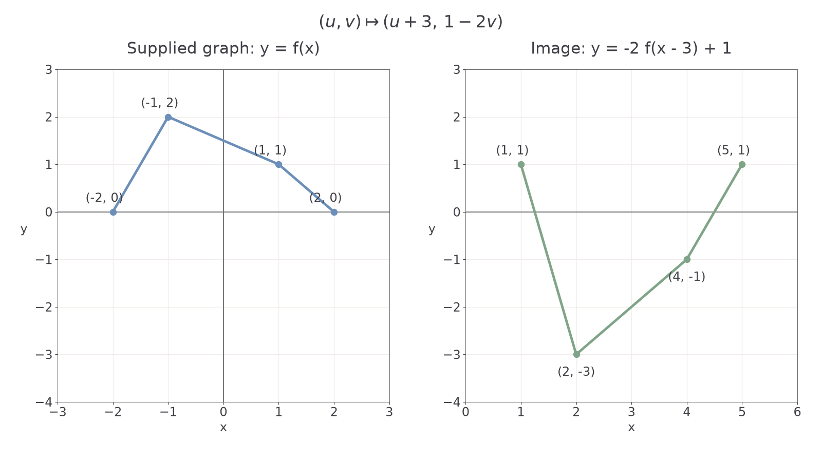
\begin{aligned} (-2,0)&\mapsto(1,1) & (-1,2)&\mapsto(2,-3) \\ (1,1)&\mapsto(4,-1) & (2,0)&\mapsto(5,1) \end{aligned}

A supplied segmented graph and its translated reflected and stretched image

Why this step? The graph is completely specified by the vertices and straight connections, so mapping those vertices determines every intervening segment too.

The first image segment has equation $y=1-4(x-1)$ ; the last has $y=-1+2(x-4)$ . Hence

\begin{aligned} 0=1-4(x-1)&\implies x=\tfrac54 && \text{first zero height} \\ 0=-1+2(x-4)&\implies x=\tfrac92 && \text{last zero height} \end{aligned}

Answer. Join the four image vertices in order, keeping the endpoints included. Domain $[1,5]$ , range $[-3,1]$ , roots $\tfrac54,\tfrac92$ . There is no $y$ -intercept because $0$ is outside the domain. Conversely, the corresponding vertices reveal the mapping $(u,v)\mapsto(u+3,1-2v)$ , so they support this sequence of transformations.

Check. Both roots lie on their claimed segments, and the two middle vertices have negative heights, so no further segment crosses the axis.

Change only the vertical multiplier, from $-2$ to $-1$ . The horizontal positions stay fixed, but the new zero heights must be found again.

Worked example 8: changing the vertical scale

Question. For the same supplied graph, describe the sketch and features of $y=-\mathrm f(x-3)+1$ .

Plan. Keep the input mapping and replace the output rule by $y=1-v$ .

\begin{aligned} (-2,0)&\mapsto(1,1) & (-1,2)&\mapsto(2,-1) \\ (1,1)&\mapsto(4,0) & (2,0)&\mapsto(5,1) \end{aligned}

The first image segment has equation $y=1-2(x-1)$ , so

0=1-2(x-1)\implies x=\tfrac32\qquad\text{find its crossing}

Why this step? Old points with height $1$ , rather than $0$ , become new roots after the reflection and upward translation.

Answer. Join $(1,1),(2,-1),(4,0),(5,1)$ in order. Domain $[1,5]$ , range $[-1,1]$ , roots $\tfrac32,4$ , and no $y$ -intercept.

Check. The vertex $(4,0)$ is a root; the last segment rises from it and introduces no additional root.

Technology can suggest patterns but a screen has boundaries. For the family $y=x^2+k$ , a plot restricted to $-1\le x\le1$ , $-1\le y\le1$ shows no part of $y=x^2-4$ . It has not disproved the roots: $x^2=4$ gives $x=\pm2$ , both outside that window. Widening it reveals them. Changing $k$ shifts every height by the same amount; the vertex $(0,k)$ explains the whole family, including values beyond a plotted grid.

For a combined family, a graphing output for $y=2(3(x-C))^2-4$ might list vertices $(0,-4),(1,-4),(2,-4)$ for $C=0,1,2$ . Interpret those coordinates: only the horizontal translation changes. The algebra $y=18(x-C)^2-4$ confirms the minimum height $-4$ , for every real $C$ , not only the three plotted choices. A table or graph supports an investigation; the equation explains its general conclusion.

Exam tip

A sketch should show the relevant features and their coordinates, not just a recognisable shape. Recalculate intercepts after a vertical translation; mapped old intercepts may no longer lie on an axis.

Use the same method on a new set of supplied straight segments. All the information needed is in the question.

Reading a newly defined curve

A short mathematical passage can define unfamiliar notation using ideas you already know. Read its permitted inputs before manipulating the formula, and translate a new term into a concrete point or graph feature.

Consider this passage:

For a positive real parameter $q$ , a cap profile is the curve

y=\mathrm C_q(u)=q-|u-q|,\qquad 0\le u\le2q

Its sides are straight. It runs from $(0,0)$ to $(q,q)$ to $(2q,0)$ , with all endpoints included. The parameter fixes the height and width together. A transformed profile applies ordinary input and output transformations to this restricted curve. No points outside its stated input interval belong to it.

For instance, when $q=3$ , $\mathrm C_3(2)=3-|2-3|=2$ . The symbol is a supplied definition, not a new formula to recall. Its shape follows because $|u-q|=q-u$ to the left of the peak and $|u-q|=u-q$ to its right.

Worked example 9: translating the profile's definition

Question. For the cap profile with $q=3$ , form an explicit equation for $y=2\mathrm C_3(x-1)-1$ . State its domain and the image of $(2,2)$ .

Plan. Replace the profile's input by $x-1$ everywhere, then impose its original input restriction.

\begin{aligned} y&=2\bigl(3-|(x-1)-3|\bigr)-1 && \text{substitute the whole input} \\ &=5-2|x-4| && \text{simplify} \\ 0\le x-1&\le6\iff 1\le x\le7 && \text{keep permitted inputs} \\ (2,2)&\mapsto(3,3) && \text{map both coordinates} \end{aligned}

Why this step? The cap's formula and its input interval belong together. Extending the formula alone would introduce points that the passage explicitly excludes.

Answer. $y=5-2|x-4|$ , domain $[1,7]$ ; the point maps onto $(3,3)$ . The peak is $(4,5)$ , and the two endpoints are $(1,-1)$ and $(7,-1)$ .

Check. At $x=3$ , the explicit formula gives $5-2|3-4|=3$ , agreeing with the mapped point.

Change only the inside scale, from $x-1$ to $2(x-1)$ . Its reciprocal halves horizontal distances before the translation.

Worked example 10: extending the passage with an input scale

Question. For the same cap, form an explicit equation for $y=2\mathrm C_3(2(x-1))-1$ . State the domain and image of $(2,2)$ .

Plan. Substitute $2(x-1)$ into the definition, then solve both the input inequality and the point equation.

\begin{aligned} y&=2\bigl(3-|2(x-1)-3|\bigr)-1 && \text{use the definition} \\ &=5-2|2x-5| && \text{collect terms} \\ 0\le2(x-1)&\le6\iff1\le x\le4 && \text{transform the domain} \\ 2(x-1)&=2\implies x=2 && \text{match the old input} \\ y&=2(2)-1=3 && \text{transform its height} \end{aligned}

Why this step? $2(x-1)=u$ gives $x=u/2+1$ ; the translation is still right $1$ , while the profile's width is halved.

Answer. $y=5-2|2x-5|$ , domain $[1,4]$ , and image point $(2,3)$ . Its peak is $(\tfrac52,5)$ .

Check. At the domain endpoints $x=1,4$ , the inside input is $0,6$ , respectively; both outputs are $-1$ , as required.

This is how to use an unfamiliar passage: identify what is defined, verify a simple case, then extend it using a familiar method. The profile definition itself is supplied here; the transformation rules are not in the formula sheet and must be known.

Watch out

Wrong: $\mathrm C_3(2(x-1))$ has domain $[0,6]$ because $\mathrm C_3$ does. Right: require $0\le2(x-1)\le6$ , giving $[1,4]$ . The input expression, not $x$ alone, must satisfy the passage's restriction.

Change only the cap parameter. The passage supplies the new height and input interval; the transformation method stays the same.

Quick Recap

Outside changes alter heights; inside changes require you to solve for the new input.
A negative scale includes a reflection, and a horizontal stretch uses the reciprocal inside multiplier.
Track a general point to respect the order of combined transformations and form the equation.
Sketch from mapped features, preserving the supplied shape and domain boundaries; find new intercepts afterwards.
A new curve definition supplies both a rule and its permitted inputs: transform both.

You can read a curve's movements from corresponding features: the segmented graph's mapping $(u,v)\mapsto(u+3,1-2v)$ reveals a right translation, reflection, vertical stretch and upward translation. The same coordinate method works for a newly defined cap profile.

Last Accessed

Pure Mathematics

Statistics

Mechanics

MC7, MC8 - Transforming and combining graphs

Changing heights by translation and stretch

Changing inputs and horizontal scale

Combining moves and forming equations

Sketching from a supplied graph

Reading a newly defined curve

Quick Recap

Learn faster with Nova