MD6–MD8 - Scatter diagrams, regression and correlation

Reading relationships in paired data

Could two groups each have an increasing trend, while their pooled scatter seems to fall? A short, slow hill route and a longer, faster flat route can make that happen.

The current LDS9 contains 200 people aged 16 and over from the American NHANES survey of 2003–04. These are individual survey records, unlike counts for whole areas. Keep the two selected columns paired by row; sorting either column alone would create different people mathematically.

In the real LDS, height and upper-arm length show a positive association. “Tend to” matters: a taller individual need not have a longer upper arm than every shorter individual. A steep gradient does not make a relationship strong: converting centimetres to metres changes the gradient, but not the tightness of the cloud.

A curved association can be pronounced while linear correlation is weak or absent. No apparent linear correlation does not establish independence. Judge the picture before choosing a model; numerical correlation coefficients and their inference are developed later.

Identify the statement that keeps those jobs separate.

Subgroups and unusual paired observations

Look for different sections of the population before committing to a single pooled description.

The left panel uses constructed cycle journeys to make the reversal visible; the right panel uses real LDS height and upper-arm measurements. The datasets are separate, as their labels and units show.

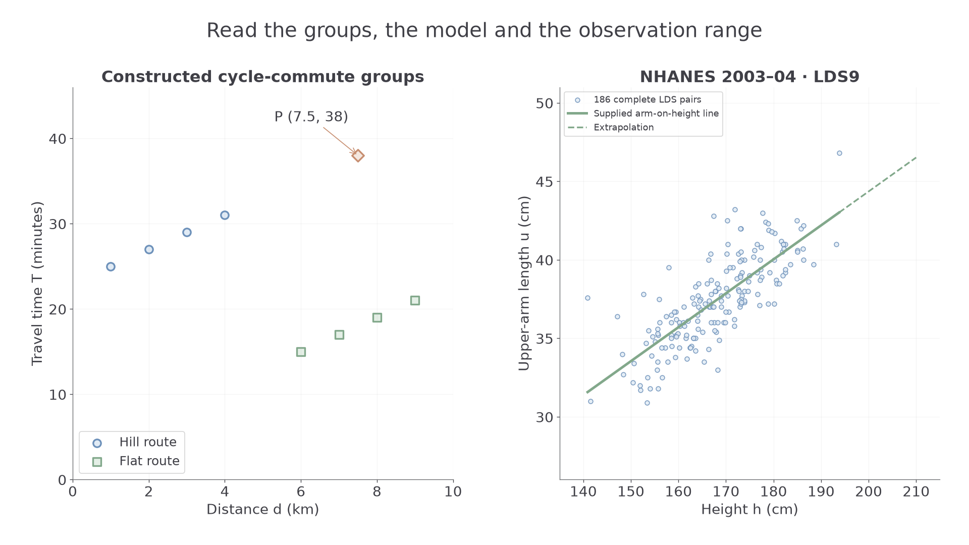
Within each route group, time increases with distance, while longer flat-route trips tend to be quicker than shorter hill-route trips. Point P at $(7.5,38)$ is inconsistent with the nearby flat-route trend. It might involve a stop or a recording issue; the picture alone cannot identify its cause.

An extreme height is not automatically a paired outlier if its arm length follows the cloud. An unusual record should be investigated, not removed merely to improve a fitted line.

Change only the flat group's times by adding 16 minutes throughout. This preserves its internal trend.

A vertical boundary around $5\,\mathrm{km}$ separates the pictured route groups without cutting through either. To add a supplied point $(4,14)$, follow the distance and time scales to their intersection. Preserve the supplied axes when making additions; numerical regression fitting is not required here.

A new pair of groups tests the same interpretation.

Using a supplied regression line

A regression line supplies predictions in a particular direction; an answer from its equation still needs a range and population check.

For the 186 LDS records with both height $h$ and upper-arm length $u$ available, software gives the line

with both measurements in cm. Observed heights range from $140.9$ to $193.8\,\mathrm{cm}$. The extra digits avoid premature rounding; report predictions below to one decimal place.

The gradient predicts about $0.216\,\mathrm{cm}$ extra upper-arm length per extra centimetre of height. The intercept is a mathematical prediction at height zero, far outside the observed range; it is not a meaningful human measurement. Rearranging the line does not turn it into the regression of height on arm length.

For example, the first LDS person's $h=173.4$ gives prediction about $38.61\,\mathrm{cm}$; the observed $37.7\,\mathrm{cm}$ has residual about $-0.91\,\mathrm{cm}$. A negative residual places that point below the line.