MR6, MR7 - Finite discrete probability distributions
Use tables and algebraic probability functions to describe finite discrete random variables. MR6 connects the variable, its values and its probability rule; MR7 uses that rule to calculate events, including uniform selections and independent observations.
Distinguish a variable from its possible values
Two devices each need 0, 1 or 2 adjustments. Could exactly one adjustment in total be more likely than none? For one device the respective probabilities are 0.40, 0.35 and 0.25. We need to distinguish an individual count from a total before answering.
You already know
An event's probability lies between 0 and 1. Add probabilities for disjoint cases. For independent events, multiply their probabilities; without independence that product need not be correct.
The experiment produces an outcome; a random variable turns that outcome into a number we can use.
Discrete random variable
A discrete random variable takes values from a set of separate possible values. Here that set, its support, is finite. Write for the variable and or for a particular value. Thus is the adjustment count, whereas is an event. A continuously measured length, with every real value in an interval possible, is a different kind of variable.
The table gives the complete probability function for one device.
| 0 | 1 | 2 | |
|---|---|---|---|
| 0.40 | 0.35 | 0.25 |
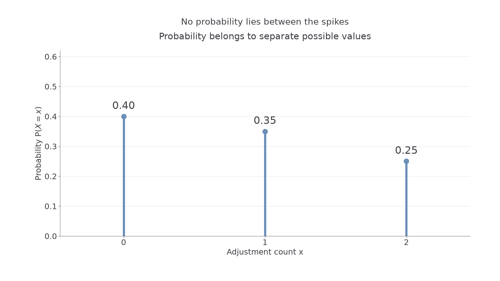
Each spike is a probability. Joining them into a continuous curve would suggest possibilities the model does not allow: for example, . The probabilities sum to 1 because exactly one listed count occurs.
Worked example 1: an inclusive count
Question. Find the probability that a device needs at most one adjustment.
Plan. Convert the words to an inequality and add the entries it permits.
Why this step? “At most” includes the stated endpoint.
Answer. The probability is 0.75.
Check. Its complement, two adjustments, has probability 0.25.
Now change only the endpoint's inclusion. The probability at 1 makes a real difference.
Worked example 2: a strict count
Question. Find the probability that a device needs fewer than one adjustment.
Plan. Keep only support values strictly below 1.
Why this step? One adjustment belongs to the previous event but not this one.
Answer. The probability is 0.40.
Check. The difference is exactly . The event still contains 0 and 1, giving 0.75.
A complete probability function describes a population of possible chance outcomes; it does not force exact proportions in every small sample.
Watch out
Wrong: . Removing the endpoint removes its probability. For a discrete distribution that probability can be positive.
Read both ends of the following interval before adding anything.
Normalise an algebraic probability rule
An algebraic probability function is a compact table: substitute each permitted value, rather than applying the formula everywhere.
Probability constraints
For a finite support ,
The probability outside is zero. Not in the formula sheet: learn it.
The total determines a normalising constant. Checking the entries afterwards protects you against algebraic solutions that cannot be probabilities.
Worked example 3: a shifted probability rule
Question. A variable has for , and zero otherwise. Determine and hence find .
Plan. Substitute every allowed value into the rule and equate their sum to 1.
Why this step? At , the coefficient is 1, not 0: the function uses .
Answer. and the probability is 0.70.
Check. The four entries are 0.1, 0.2, 0.3 and 0.4, all valid and totalling 1. Value 4 is outside the support, so its probability is zero.
Extend only the support, adding the value 4. The same formula must now share total probability among five entries.
Continue this lesson.
You’re previewing NovaLearn without an account. Create a free account to read the rest.
Create free account