MR8 - Choosing distributions and the normal approximation

Shape and support determine model suitability

How can a Normal curve approximate a positive probability at one count when its probability at one point is zero? Consider sixty independent fair coin tosses. Exactly thirty heads has probability about $0.103$, yet a continuous Normal variable satisfies $\mathrm P(Y=30)=0$. The answer will be an area around thirty, rather than the point itself.

Before finding an area, ask whether one Normal curve represents the distribution sensibly. A roughly symmetric, bell-shaped histogram of a continuous measurement supports it. A long right tail or two separate peaks gives evidence against it. The measurement's physical range matters too: impossible-value tails must be negligible for the task.

A binomial count remains discrete, but a near-symmetric bell-shaped count distribution may be approximated by a Normal curve. Compare these two distributions. They have the same number of trials, but very different shapes.

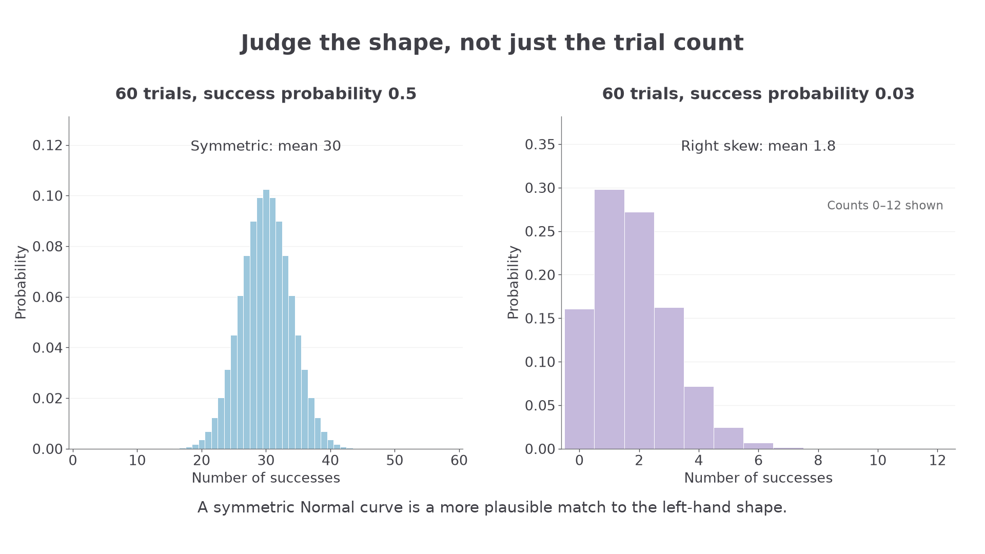
Sixty trials do not settle the choice: one distribution is symmetric, while the other is crowded against zero.

For $X\sim\mathrm B(60,0.5)$, a supplied matching approximation is $Y\sim\mathrm N(30,15)$. The second parameter is variance, so the standard deviation is $\sqrt{15}$. The count boundaries $0$ and $60$ are each about $7.75$ standard deviations from the mean; the shape and remote boundaries support the approximation.

For $\mathrm B(60,0.03)$, the supplied mean and standard deviation are $1.8$ and approximately $1.32$. The distribution is right skewed and close to its lower boundary. A symmetric curve would spill into negative counts near its centre. Changing only the success probability can therefore undermine the approximation.

MEI asks you to recognise this from the shape, not to memorise numerical conditions involving the binomial parameters. In this lesson the matching Normal parameters are supplied; the variance formula for a binomial is not printed on the MEI formula sheet.

That distinction also applies to mixtures. Combining two groups can create two peaks even if each group separately looks Normal.

Give each integer count a unit-width interval

Give each integer its own interval of width one. Then a probability at one count can be represented by an area.

For count $24$, draw a bar from $23.5$ to $24.5$, with height $\mathrm P(X=24)$. Its width is one, so its area equals that probability. The neighbouring bars meet at half-integers. A smooth curve approximates their areas, not their heights at isolated points.

The picture shades every bar for counts twenty through twenty-four, so the two outside edges are $19.5$ and $24.5$.

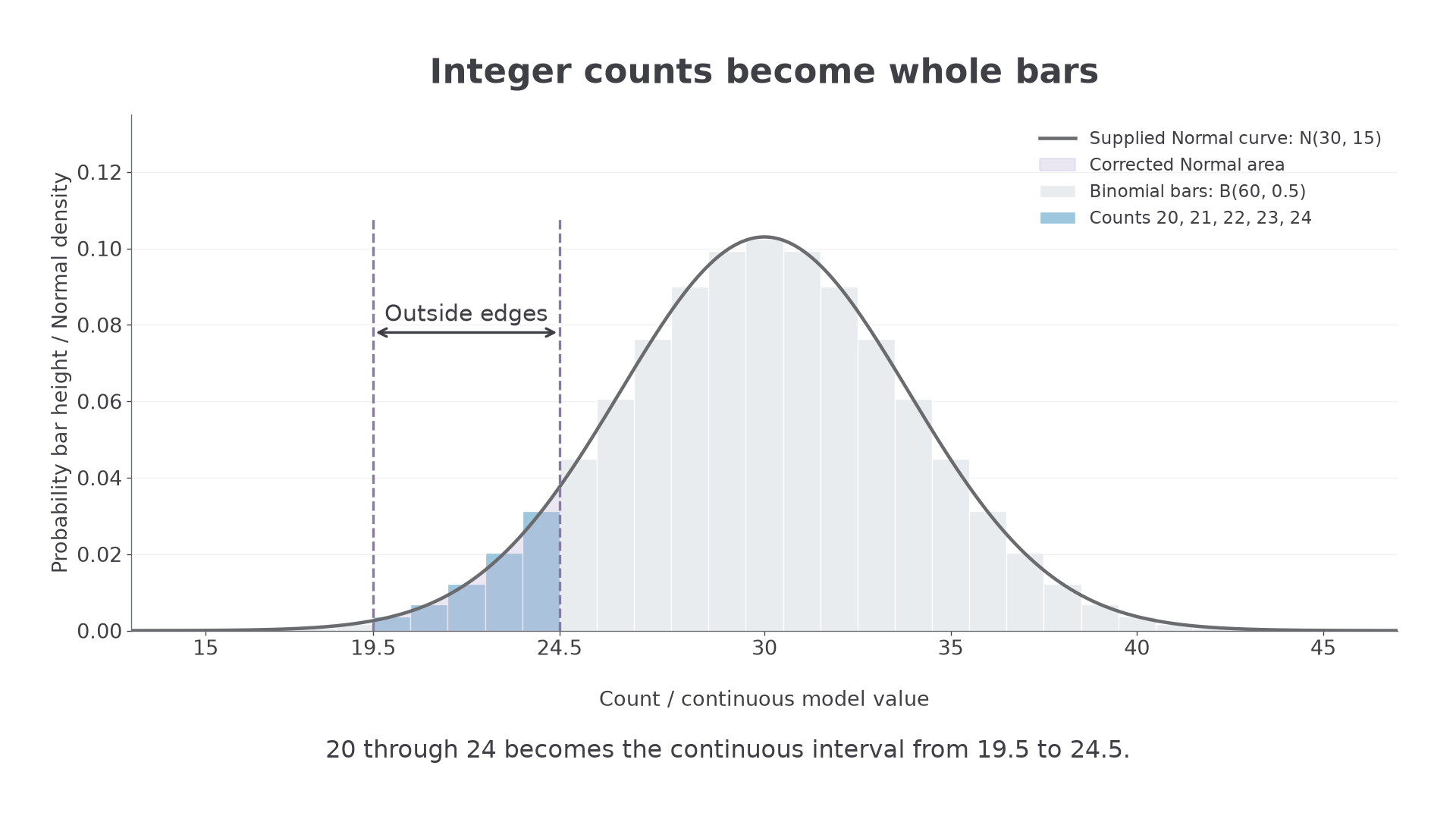
Include whole bars at the boundary counts. The smooth area between the outside edges approximates their total probability.

Here are the boundary choices for one cutoff. In each row, find the last or first included integer before moving half a unit outwards.