Mk7, Mk8 - Constant acceleration formulae | OCR A-Level Mathematics B (MEI)

Recognise a constant-acceleration interval, derive its five scalar relationships and choose a useful equation. Solve staged straight-line and vertical-motion problems while checking directions, time roots and the limits of the model.

When the formulae apply

If you double a ball's upward launch speed, do you double the height it rises? Under a constant-gravity model the rise actually quadruples. With $g=9.8\,\mathrm{m\,s^{-2}}$ , launches at $9.8$ and $19.6\,\mathrm{m\,s^{-1}}$ rise $4.9$ and $19.6\,\mathrm m$ . We will explain the square hiding in that comparison.

You already know

Velocity and displacement carry signs. Speed and distance do not. A straight velocity-time line has constant gradient, while its signed area gives displacement.

Choose a positive direction and an interval start. Write $u$ for initial velocity, $v$ for velocity after elapsed time $t$ , $a$ for acceleration and $s$ for displacement during this interval. Absolute position would also need the starting coordinate.

Constant acceleration

Equal elapsed times produce equal signed changes in velocity. A velocity-time graph is therefore a straight line. Zero acceleration is allowed; reversing velocity is also allowed without changing the acceleration.

For instance, $v=6-2t$ changes by $-2\,\mathrm{m\,s^{-1}}$ each second. The velocity becomes negative after $3\,\mathrm s$ , but acceleration stays $-2\,\mathrm{m\,s^{-2}}$ . In contrast, $v=6-t^2$ has changing gradient $-2t$ . One constant-acceleration model cannot cover that motion.

Keep units consistent, usually metres and seconds. A staged journey needs separate elapsed times when acceleration changes. An impact or bounce also begins a new interval. An average acceleration does not generally reproduce the correct displacement.

Key idea

Recognising the model comes before choosing the formula: one line of motion, one interval and one constant signed acceleration.

Test the distinction between a constant gradient and a constant graph height.

Deriving the five relationships

The supplied equations share one source: the straight-line velocity graph.

[DIAGRAM: asset_name: Constant acceleration velocity graph; asset_slug: suvat_derivation; description: Straight velocity-time line from initial velocity u to final velocity v over elapsed time t, with rectangle ut and triangular area one half (v-u)t; caption: Constant acceleration velocity graph]

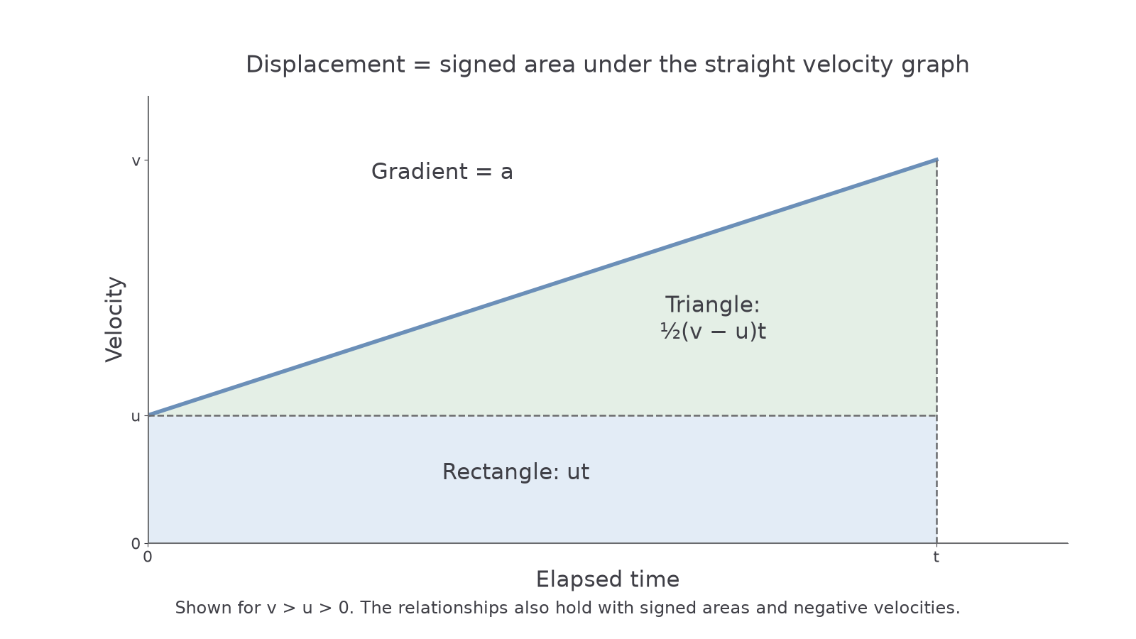
Its gradient gives $a=(v-u)/t$ , so $v=u+at$ . Its signed area gives $s=\frac12(u+v)t$ . If a segment crosses the time axis, this area still gives displacement because the below-axis contribution is negative.

Constant-acceleration relationships

For straight-line motion with constant signed $a$ ,

\begin{aligned} v&=u+at\\ s&=ut+\tfrac12at^2\\ s&=vt-\tfrac12at^2\\ s&=\tfrac12(u+v)t\\ v^2-u^2&=2as \end{aligned}

All quantities must refer to the same interval; $s$ denotes displacement.

In the formula sheet.

You should be able to derive the relationships, even though they are supplied. Start by eliminating an endpoint velocity.

Worked example 1: retain the initial velocity

Question. Use $v=u+at$ and $s=\frac12(u+v)t$ to derive a displacement equation containing $u,a,t$ .

Plan. Replace the unknown final velocity in the area formula.

\begin{aligned} s&=\tfrac12(u+u+at)t &&\text{substitute }v\\ &=\tfrac12(2u+at)t &&\text{collect}\\ &=ut+\tfrac12at^2 &&\text{expand} \end{aligned}

Why use this substitution? It removes the endpoint velocity absent from the requested equation.

Answer. $s=ut+\frac12at^2$ , for constant acceleration.

Check. The terms $ut$ and $at^2$ both have displacement units.

Change only the retained endpoint velocity from $u$ to $v$ ; the starting relationships remain the same.

Worked example 2: retain the final velocity

Question. Use $v=u+at$ and $s=\frac12(u+v)t$ to derive a displacement equation containing $v,a,t$ .

Plan. Rearrange first so that the initial velocity can be removed.

\begin{aligned} u&=v-at &&\text{rearrange}\\ s&=\tfrac12(v-at+v)t &&\text{substitute }u\\ &=\tfrac12(2v-at)t &&\text{collect}\\ &=vt-\tfrac12at^2 &&\text{expand} \end{aligned}

Why subtract half the acceleration term? The final velocity is not the average over an accelerating interval.

Answer. $s=vt-\frac12at^2$ , for constant acceleration.

Check. Putting $v=u+at$ into the result returns the first equation.

The remaining relationship follows without dividing by $a$ :

v^2-u^2=(v-u)(v+u)=at(v+u)=2as

The factorisation therefore remains valid when $a=0$ . An integration route begins with constant $a$ :

\begin{aligned} v(\tau)&=a\tau+C,\qquad v(0)=u\ \Rightarrow\ C=u &&\text{integrate and use initial velocity}\\ s&=\int_0^t(u+a\tau)\,\mathrm d\tau =ut+\tfrac12at^2 &&\text{signed displacement} \end{aligned}

Here $\tau$ is just an integration variable. The displacement starts at zero; an absolute position needs its initial offset. These derivations are not in the formula sheet.

Watch out

Wrong: “ $s=\frac12(u+v)t$ works for every velocity function.” Correct: endpoint averaging gives displacement for a linear velocity function, not a general curve.

Now derive the relationship which removes time.

Choose the equation and interval

List the known quantities for one stage, then select a relationship which omits an unneeded variable.

If this quantity is absent	Useful equation
Displacement	$v=u+at$
Final velocity	$s=ut+\frac12at^2$
Initial velocity	$s=vt-\frac12at^2$
Acceleration	$s=\frac12(u+v)t$
Time	$v^2-u^2=2as$

The equations in the table are supplied. If $v^2$ is found, choose the velocity sign from the physical direction. If a quadratic gives two times, check the interval before retaining either.

Worked example 3: slowing then cruising

Question. A train moving forwards at $18\,\mathrm{m\,s^{-1}}$ slows with constant acceleration $-1.5\,\mathrm{m\,s^{-2}}$ to $9\,\mathrm{m\,s^{-1}}$ , then cruises at that velocity for $8\,\mathrm s$ . Determine total time and distance.

Plan. Find the braking duration and area, then add the constant-velocity stage.

\begin{aligned} t_1&=(9-18)/(-1.5)=6 &&\text{velocity change}\\ s_1&=\tfrac12(18+9)(6)=81 &&\text{braking displacement}\\ s_2&=9(8)=72 &&\text{cruising displacement}\\ T&=6+8=14,\qquad D=81+72=153 &&\text{positive motion throughout} \end{aligned}

Why not use one acceleration? The cruising stage has acceleration zero.

Answer. Total time $14\,\mathrm s$ , distance $153\,\mathrm m$ .

Check. Braking speed lies between $9$ and $18$ , so its $81\,\mathrm m$ travel lies between $54$ and $108\,\mathrm m$ .

Continue this lesson.

You’re previewing NovaLearn without an account. Create a free account to read the rest.

Create free account

Last Accessed

Pure Mathematics

Statistics

Mechanics

Mk7, Mk8 - Constant acceleration formulae

When the formulae apply

Deriving the five relationships

Choose the equation and interval

Continue this lesson.

Learn faster with Nova