ME7 - Linearising power and exponential models | OCR A-Level Mathematics B (MEI)

Choose coordinates that make a power or exponential model look straight, then recover the model from the line. Use fitted experimental graphs, read logarithmic scales and follow a short argument in newly defined coordinates, keeping the meaning of every parameter in view.

Turning a power model into a line

Can a straight line describe measurements that follow a curve? Consider $y=6\sqrt{x}$ : at $x=1,4,9$ , the outputs are $6,12,18$ . The input steps are unequal, but doubling $\sqrt{x}$ doubles $y$ . Logarithms reveal the power relationship without requiring you to guess it.

You already know

For positive arguments, $\log_{10}(uv)=\log_{10}u+\log_{10}v$ and $\log_{10}(x^n)=n\log_{10}x$ . A line has form $Y=mX+c$ , and $10^c$ reverses a base-ten logarithm.

Here is a useful surprise: the gradient of a log-log power plot is unchanged if you switch from common logs to natural logs. Both coordinates are rescaled by the same factor. The intercept changes, so its inverse still needs the correct base.

Linearisation

Linearisation rewrites a relationship as a straight-line equation in new coordinates. For a power model with positive inputs and outputs, put $X=\log_{10}x$ and $Y=\log_{10}y$ . Approximate straightness supports a power model; it does not prove that the model is the physical cause.

Take logarithms of the whole right-hand side, including its coefficient.

Power-model coordinates

For $y=ax^n$ , with $a>0$ , $x>0$ and $n$ real,

\begin{aligned} \log_{10}y&=\log_{10}a+n\log_{10}x\\ Y&=nX+\log_{10}a \end{aligned}

Hence gradient $m=n$ , intercept $c=\log_{10}a$ , and $a=10^c$ . With natural logs, use $a=\mathrm e^c$ .

Not in the formula sheet: learn it.

Positive outputs can have negative logarithms. For example, $\log_{10}0.1=-1$ ; the input to the logarithm remains positive.

Worked example 1: reading a positive power

Question. A fitted line is $\log_{10}y=0.5\log_{10}x+\log_{10}6$ . Determine the model and its value at $x=9$ .

Plan. Compare with the transformed power equation and undo its intercept.

\begin{aligned} n&=0.5 &&\text{compare gradients}\\ a&=10^{\log_{10}6}=6 &&\text{undo the intercept}\\ y(9)&=6(9^{1/2})=18 &&\text{use the recovered model} \end{aligned}

Why this step? The intercept is $\log_{10}6$ , whereas the coefficient of the model is $6$ .

Answer. $y=6x^{1/2}$ , giving $y=18$ at $x=9$ .

Check. $\log_{10}18=0.5\log_{10}9+\log_{10}6$ , by the log laws.

Change only the sign of the gradient. A decreasing power is still compatible with positive log arguments.

Worked example 2: reading a negative power

Question. A fitted line is $\log_{10}y=-0.5\log_{10}x+\log_{10}6$ . Determine the model and its value at $x=9$ .

Plan. Keep the same coefficient and read the signed exponent.

\begin{aligned} n&=-0.5 &&\text{retain the negative sign}\\ a&=6 &&\text{the intercept is unchanged}\\ y(9)&=6(9^{-1/2})=2 &&\text{evaluate the negative power} \end{aligned}

Why this step? A negative gradient describes a negative exponent; it does not make the output negative.

Answer. $y=6x^{-1/2}$ , giving $y=2$ at $x=9$ .

Check. From $x=1$ to $x=9$ , the output is multiplied by $9^{-1/2}=1/3$ .

When a physical variable is logged, use its numerical value in fixed stated units, such as $\log_{10}(t/(1\,\mathrm{s}))$ . Keep those units when recovering the coefficient. Investigate zero or negative readings rather than deleting them to make a graph work.

Watch out

From $Y=nX+c$ , writing $y=cx^n$ loses the inverse transformation. For base-ten coordinates, the coefficient is $10^c$ .

Use the line's coefficients to recover a new decreasing model.

Turning an exponential model into a line

An exponential model multiplies its output by a fixed factor for each unit increase in its input. Log only the output, leaving the input unchanged.

Exponential-model coordinates

For $y=ab^x$ , where $a>0$ and $b>0$ ,

\log_{10}y=\log_{10}a+x\log_{10}b.

A plot of $\log_{10}y$ against $x$ has gradient $m=\log_{10}b$ and intercept $c=\log_{10}a$ . Hence $b=10^m$ , $a=10^c$ . With natural logs use $b=\mathrm e^m$ , $a=\mathrm e^c$ .

Not in the formula sheet: learn it.

The signs tell you about change: positive gradient gives $b>1$ , negative gradient gives $0<b<1$ , and zero gradient gives $b=1$ , a constant output. In $y=a\mathrm e^{kx}$ , a natural-log plot's gradient is directly $k$ .

Worked example 3: growth from a natural-log line

Question. A line fitted to $\ln y$ against $x$ is $\ln y=0.20x+\ln5$ . Determine $a$ and $b$ in $y=ab^x$ .

Plan. Compare the intercept and gradient, then reverse their natural logs.

\begin{aligned} a&=\mathrm e^{\ln5}=5 &&\text{recover the coefficient}\\ b&=\mathrm e^{0.20}\approx1.2214 &&\text{recover the multiplier}\\ y&=5\mathrm e^{0.20x} &&\text{write an equivalent model} \end{aligned}

Why this step? The gradient $0.20$ is $\ln b$ , not the multiplier $b$ .

Answer. $a=5$ , $b=\mathrm e^{0.20}$ ; thus $y=5(\mathrm e^{0.20})^x$ .

Check. Increasing $x$ from $0$ to $1$ multiplies $y$ by $\mathrm e^{0.20}$ , giving $y(1)\approx6.107$ .

Change only the sign of the gradient. The initial coefficient remains the same, while the multiplier becomes less than $1$ .

Worked example 4: decay from the same intercept

Question. A fitted line is $\ln y=-0.20x+\ln5$ . Determine its exponential model.

Plan. Exponentiate the signed gradient and the unchanged intercept.

\begin{aligned} a&=5 &&\text{same intercept}\\ b&=\mathrm e^{-0.20}\approx0.81873 &&\text{undo the negative log}\\ y&=5\mathrm e^{-0.20x} &&\text{recover the relationship} \end{aligned}

Why this step? A negative logarithm gives a positive multiplier between $0$ and $1$ ; a negative multiplier would not define this real exponential for all real inputs.

Answer. $y=5(\mathrm e^{-0.20})^x$ , a decay model.

Check. At $x=1$ , $y\approx4.094$ , which is positive and less than its value $5$ at $x=0$ .

Common-log axes require powers of $10$ instead. Keep the input coordinate unchanged in either case.

Watch out

A straight plot of $\log_{10}y$ against $x$ with gradient $m$ gives base $10^m$ . The same numerical gradient on a natural-log plot gives base $\mathrm e^m$ ; these are different models.

The next line uses common logs, so select its inverse carefully.

Estimating from fitted graphs

Measurements usually scatter. Use the pattern of all transformed points, rather than expecting every one to sit exactly on a line.

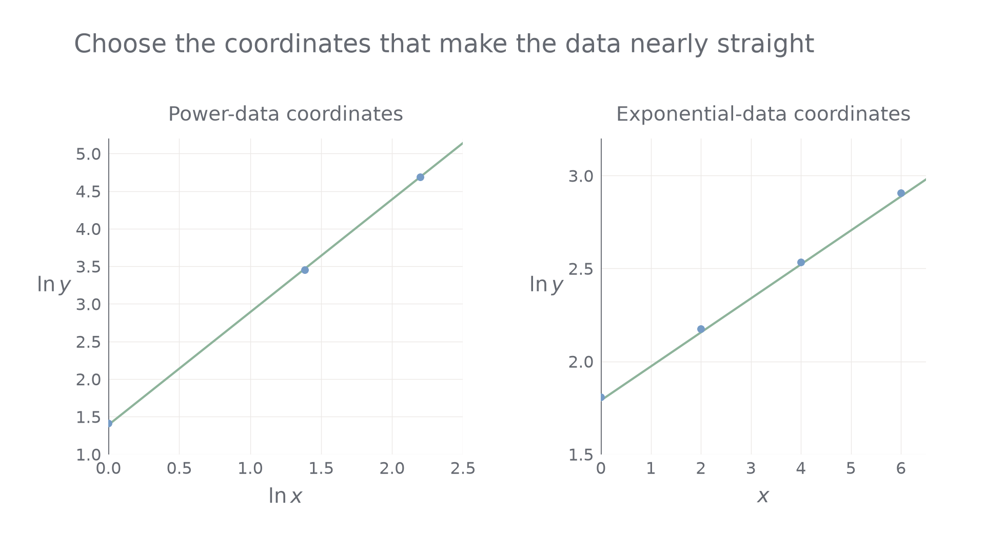
Transformed experimental data with approximate fitted lines for a power model and an exponential model

The two experiments need different horizontal coordinates. The left-hand gradient is a power; the right-hand gradient is a logarithm of an exponential multiplier.

For the power experiment, $x=1,4,9$ and $y=4.1,31.7,108.5$ , giving rounded natural-log pairs $(0,1.411)$ , $(1.386,3.456)$ , $(2.197,4.687)$ . An approximate fitted line is $Y=1.50X+1.39$ . For the exponential experiment, $x=0,2,4,6$ and $y=6.1,8.8,12.6,18.3$ ; its approximate line is $\ln y=0.183x+1.79$ .

Enter paired data together, calculate the appropriate log columns and inspect the scatter. A calculator's linear-regression function must use those transformed columns, not simply the untransformed measurements. Keep unrounded logs in the calculation. Read or fit a line using all points, then use two well-separated points on that line for a gradient calculation. Points on the fitted line need not be experimental readings.

Worked example 5: a line with its intercept visible

Question. A fitted line on axes $X=\ln x$ , $Y=\ln y$ passes through $(0,1.39)$ and $(2,4.39)$ . Determine a model for $y$ .

Plan. Find the gradient, identify the intercept and compare with the power transformation.

\begin{aligned} m&=\frac{4.39-1.39}{2-0}=1.50 &&\text{rise over run}\\ c&=1.39 &&\text{read the height at }X=0\\ a&=\mathrm e^{1.39} &&\text{undo the natural log}\\ y&=\mathrm e^{1.39}x^{1.50} &&\text{use }n=m \end{aligned}

Why this step? Here $X=0$ means $x=1$ , not $x=0$ .

Answer. $y\approx4.01x^{1.50}$ .

Check. The unrounded model gives $y(4)\approx32.1$ , about $1.32\%$ above the measurement $31.7$ . Small scatter is compatible with an approximate fit.

Change only the horizontal transformation: the following fitted line uses the input itself. Its gradient now has a different meaning.

Worked example 6: the same line on different axes

Question. A fitted line through $(0,1.39)$ and $(2,4.39)$ is drawn on axes $x$ and $\ln y$ . Determine a model for $y$ .

Plan. Use the same line calculation, then compare with the exponential transformation.

\begin{aligned} m&=1.50 &&\text{the line coordinates are unchanged}\\ \ln a&=1.39 &&\text{read the intercept}\\ \ln b&=1.50 &&\text{interpret the new horizontal axis}\\ y&=\mathrm e^{1.39}(\mathrm e^{1.50})^x &&\text{recover the model} \end{aligned}

Why this step? The axes determine what a slope measures; the number $1.50$ alone cannot identify a model.

Answer. $y=\mathrm e^{1.39+1.50x}$ .

Check. At $x=2$ , $\ln y=4.39$ , the second line point.

Continue this lesson.

You’re previewing NovaLearn without an account. Create a free account to read the rest.

Create free account

Last Accessed

Pure Mathematics

Statistics

Mechanics

ME7 - Linearising power and exponential models

Turning a power model into a line

Turning an exponential model into a line

Estimating from fitted graphs

Continue this lesson.

Learn faster with Nova