MD1–MD5 - Univariate diagrams, histograms and distributions
Choose and read single-variable displays in MD1, use histogram area in MD2 and cumulative frequency in MD3, and describe distribution shape in MD4. MD5 explains what larger unbiased samples can improve. The current health large data set gives us real observations to investigate.
Data types determine the display
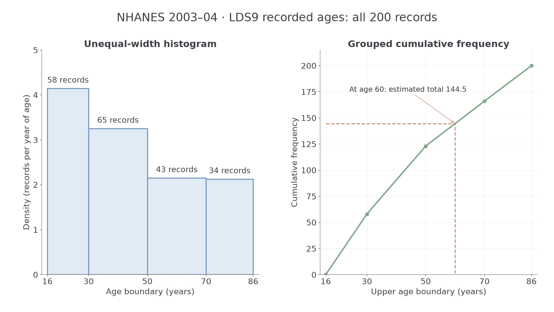
Can a wider, shorter histogram bar contain more observations? The current large data set records 58 people aged 16–29 and 65 aged 30–49: the second band contains more people, but spreads them over more years.
You already know
A frequency counts observations; a proportion divides that count by the relevant total. A graph's key tells you what each mark represents.
These are data from 200 people aged 16 and over in the American NHANES survey of 2003–04, supplied as LDS9 for the June 2027 examination. They are a small extract of a health survey, not a census and not a description of today's UK population.
Types of data
Categorical data record categories, such as marital status. Discrete numerical data take separate values, such as a count of measurements. Continuous numerical data measure quantities that can vary throughout an interval, such as height. Ranked data record order without necessarily measuring equal gaps between ranks.
The LDS records age in completed years, so that recorded variable has integer values; exact age and height are continuous quantities. Rounded height readings do not make underlying height a count. “Married” and “widowed” are categories, without a natural numerical order. First and second in a height ranking reveal order, but not whether their heights differ by or .
A categorical bar chart separates bars; a vertical line chart can show discrete numerical values. A frequency chart has equal-width numerical classes and frequency on its vertical axis. A histogram uses area proportional to frequency, which also works for unequal class widths.
Key idea
Ask what the values mean before choosing the display. Numerical category codes and ranks do not turn labels into measurements with equal gaps.
That distinction matters more than the number of decimal places a spreadsheet happens to show.
Reading single-variable displays
A display can retain actual values, combine them into classes, or reduce them to a handful of summaries.
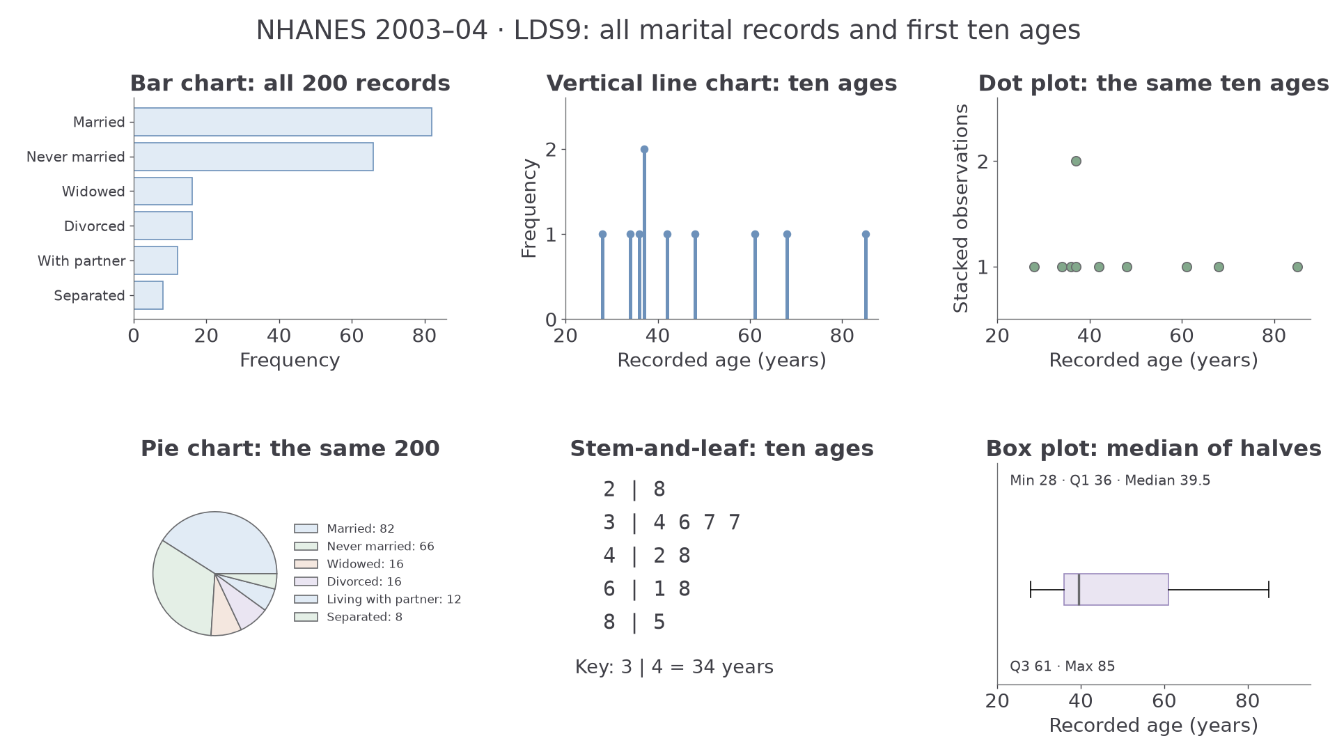
The diagram uses real LDS marital-status counts for all 200 people and the first ten recorded ages for its small numerical displays. Different panels deliberately answer different questions.
| Display | What to inspect | What it reveals or hides |
|---|---|---|
| Bar chart or pie chart | Categories, frequencies or proportions | Compares categories; pie angles show parts of one whole. |
| Vertical line chart or dot plot | Numerical positions and heights or stacks | Preserves discrete values and repeats. |
| Stem-and-leaf | Stem, every leaf and the key | Retains actual values; a repeated leaf is another person. |
| Box plot | Median, quartiles and stated whisker rule | Summarises position and spread; hides detailed peaks and sample size. |
| Equal-width frequency chart | Class boundaries and frequency axis | Heights are counts because widths agree; a density axis means something different. |
For example, the 82 married people occupy proportion , giving a pie angle of . Comparative pie-chart areas proportional to frequency are not required here. Adding a missing bar, point or leaf to a supplied diagram must use its existing scale and key.
Worked example 1: reading real ages
Question. The first ten recorded LDS ages are shown as , , , , , with key years. Find the proportion aged at least 40.
Plan. Decode the leaves, keeping repeats, and count those meeting the boundary.
Why keep both 37s? They represent two different records.
Answer. , or , of this ten-record extract.
Check. Five ages are below 40 and five are not; all ten are accounted for.
Change only the age threshold; the records and key stay fixed.
Worked example 2: moving the age boundary
Question. For the same ten recorded ages, find the proportion aged at least 60.
Plan. Count qualifying leaves at stems 6 and above.
Why retain the denominator? Moving the threshold changes the selected group, not the number of records studied.
Answer. , or , of the extract.
Check. Moving the boundary upwards has reduced the count from five to three.
Read axes as critically as keys. Counts of 100 and 110 differ by relative to 100; an axis starting at 95 shows visible heights 5 and 15 and can exaggerate the difference. A box whose median lies near one end still contains approximately a quarter of the data between that median and each neighbouring quartile.
Watch out
A graph can make a correct pair of numbers look dramatically different. State the labelled counts or proportions rather than using an apparent bar-height ratio from a truncated axis.
A small new set checks the same reading skill without requiring memorised LDS values.
Histogram area represents frequency
The first two LDS age classes answer our opening puzzle: the band with more people need not have the taller bar.
Frequency density
Frequency density is frequency per unit class width. In a histogram with a frequency-density axis, bar area equals frequency; more generally, bar area is proportional to frequency according to the stated area scale.
All 200 recorded ages are available. Grouping the recorded integer values gives the following table. The graph describes the age values stored in this extract; it does not recover precision beyond the recorded data.
| Age , years | Frequency | Width | Density |
|---|---|---|---|
| 58 | 14 | ||
| 65 | 20 | ||
| 43 | 20 | ||
| 34 | 16 |
The last boundary contains every recorded age; this is a display of recorded data, not a claim about the survey's treatment of all possible ages.
Histogram frequency and proportion
For a frequency-density axis:
Widths must be positive. The proportion estimates a probability for a suitably represented population; it is exactly the proportion of the displayed records.
Not in the formula sheet: learn it.
The diagram keeps the unequal widths visible, alongside cumulative totals for the same records.
Worked example 3: recovering a frequency
Question. A histogram class has width 20 years and frequency density people per year of age. Find its frequency.
Plan. Multiply its two dimensions, retaining the units.
Why multiply? The density gives a count per year, so multiplying by years gives a count.
Answer. people.
Check. , the supplied height.
Change only the vertical scale: the plotted height is unchanged, but one unit of plotted area now represents two people.
Worked example 4: using an area scale
Question. A bar has width 20 and plotted height . Each unit of plotted area represents two people. Find its frequency.
Plan. Find plotted area, then apply the stated conversion.
Why is 65 insufficient? The vertical axis is a plotted scale, not ordinary frequency density.
Answer. people.
Check. The answer doubles when the area-to-frequency conversion doubles.
Continue this lesson.
You’re previewing NovaLearn without an account. Create a free account to read the rest.
Create free account