Mg16 - Parametric models and restricted parameters | OCR A-Level Mathematics B (MEI)

Construct and interpret parametric models, including the kinematics and projectile contexts in Mg16. You will choose physical domains, compare observations with predictions, and explain why a curve on its own does not specify the timing of a journey.

Constructing a model with a shared parameter

When does an algebraically correct point stop belonging to a model? In a flight model, a negative height after landing may satisfy the equations perfectly. In a rectangle model, a zero side may satisfy the perimeter equation perfectly. The domain decides which predictions have a physical meaning.

Start with a rectangle of perimeter $20\,\mathrm{cm}$ : width $3\,\mathrm{cm}$ gives height $7\,\mathrm{cm}$ . Width $7\,\mathrm{cm}$ gives height $3\,\mathrm{cm}$ . Both areas are $21\,\mathrm{cm^2}$ ; the family contains a useful symmetry.

You already know

A shared parameter supplies all coordinates or quantities at the same value. Eliminating it preserves a path only if you also preserve the domain and any branch restrictions.

A modelling statement needs meanings and units. The parameter might be a side length rather than time.

Parametric model

A parametric model describes related quantities using one parameter, together with its interpretation, units, assumptions and permitted domain. Algebraic solutions outside that domain are not predictions of the stated situation.

The perimeter constraint is exact for an ideal rectangle; the choice of parameter controls how the same family is labelled.

Worked example 1: width as the parameter

Question. A rectangle has perimeter $20\,\mathrm{cm}$ . Using width $t$ centimetres, model width $x$ , height $y$ and area $A$ , with the permitted domain.

Plan. Use the perimeter to link the sides and require each to be positive.

\begin{aligned} x+y&=10 &&\text{halve the perimeter equation}\\ x&=t,\quad y=10-t &&\text{width parameter}\\ A&=t(10-t),\quad0<t<10 &&\text{area and positive sides} \end{aligned}

Why this step? A zero side would give a degenerate shape, even though its perimeter equation still holds.

Answer. The stated equations with $0<t<10$ describe the rectangle family; $A$ is measured in square centimetres.

Check. At $t=3$ , the sides are $3,7$ , the perimeter is $20$ and the area is $21$ .

Change only the parameter's meaning: let $u$ be the height instead. The physical family stays fixed.

Worked example 2: height as the parameter

Question. Describe the same rectangles using height $u$ centimetres. Relate $u$ to the previous parameter.

Plan. Make $y=u$ and solve the same perimeter constraint for $x$ .

\begin{aligned} y&=u,\quad x=10-u &&\text{same perimeter}\\ A&=u(10-u),\quad0<u<10 &&\text{area and domain}\\ u&=10-t &&\text{same rectangle in both models} \end{aligned}

Why this step? Equal parameter values need not select the same rectangle when the parameter's meaning has changed.

Answer. $x=10-u$ , $y=u$ , $A=u(10-u)$ , $0<u<10$ , with $u=10-t$ .

Check. The width- $3$ rectangle has $u=7$ , producing $(x,y)=(3,7)$ again.

Increasing one side by $1\,\mathrm{cm}$ decreases the other by $1\,\mathrm{cm}$ . The algebra describes their linked changes without treating the parameter as seconds. These models are derived from perimeter and area; they are not in the formula sheet.

Watch out

Wrong: a model with $y=u$ still has $x=u$ . Right: preserve the physical constraint, giving $x=10-u$ . Define what your parameter represents before substituting.

Try a new perimeter while retaining height as the parameter.

Time, position and average changes

A time model retains information that disappears from a Cartesian path. Initial coordinates locate the start; coordinate changes per second describe how the position develops.

Average coordinate change per unit time

For $t_1\ne t_2$ ,

\text{average }x\text{-rate}=\frac{x(t_2)-x(t_1)}{t_2-t_1},\qquad \text{average }y\text{-rate}=\frac{y(t_2)-y(t_1)}{t_2-t_1}.

Use position and time units consistently. Not in the formula sheet: learn it.

Constant coefficients in linear coordinate-time equations give the same rates over every allowed interval. A constant vertical rate is a modelling assumption, not a property of all paths.

Worked example 3: a robot's timed path

Question. A robot's position is $x=1+2t$ , $y=6-t$ , $0\le t\le5$ , in metres and seconds. Find its position at $t=3$ , its average coordinate rates and its Cartesian path.

Plan. Substitute for the position, read the constant changes and eliminate time.

\begin{aligned} t=3&:\ (x,y)=(7,3) &&\text{same time in both equations}\\ \Delta x/\Delta t&=2,\quad\Delta y/\Delta t=-1 &&\text{linear coordinate changes}\\ t&=\frac{x-1}{2} &&\text{recover time}\\ y&=\frac{13-x}{2},\quad1\le x\le11 &&\text{path and domain} \end{aligned}

Why this step? A negative coordinate rate means movement in the negative coordinate direction; it is not a negative time.

Answer. The position is $(7,3)$ , the average rates are $2$ and $-1\,\mathrm{m\,s^{-1}}$ , and the path is the stated segment.

Check. The endpoint positions $(1,6)$ , $(11,1)$ give rates $10/5=2$ , $-5/5=-1$ .

Change only the time origin by defining $u=t-2$ , measured in seconds.

Worked example 4: translate the observation clock

Question. Express the same journey in terms of $u=t-2$ , giving its domain and the position at $u=0$ .

Plan. Substitute $t=u+2$ throughout the model and interval.

\begin{aligned} x&=1+2(u+2)=5+2u &&\text{new time origin}\\ y&=6-(u+2)=4-u &&\text{same replacement}\\ -2&\le u\le3 &&\text{translated interval}\\ u=0&:\ (5,4) &&\text{old time }t=2 \end{aligned}

Why this step? The start of the journey and the zero of a clock need not coincide.

Answer. $x=5+2u$ , $y=4-u$ , $-2\le u\le3$ ; the position at $u=0$ is $(5,4)$ .

Check. At $u=-2$ , the position is $(1,6)$ , the unchanged start.

The earlier boat model $x=2+3t$ , $y=1+2t$ , $0\le t\le4$ , works in the same way: it starts at $(2,1)$ , ends at $(14,9)$ , and its average coordinate rates are $3$ and $2\,\mathrm{m\,s^{-1}}$ . These timed paths are derived models, not formula-sheet entries.

Watch out

Wrong: copying $0\le u\le5$ after changing the time origin. Right: translate the interval with the same relation used in the equations.

Shift the robot's clock by a different amount.

A projectile path with a physical domain

For a supplied flight model, use the meaning of the coordinates to set the domain. Here $x$ is horizontal distance in metres, $y$ is height above level ground in metres and $t$ is seconds after launch. Assume a point object, constant downward gravitational acceleration and negligible air resistance during the flight.

[DIAGRAM: asset_name: A restricted projectile model; caption: A restricted projectile model; asset_slug: h640-projectile-path; description: The path x equals 10t and y equals 9.8t minus 4.9t squared for 0 to 2 seconds, with launch, landing, peak at 10 comma 4.9 and two equal-height positions labelled]

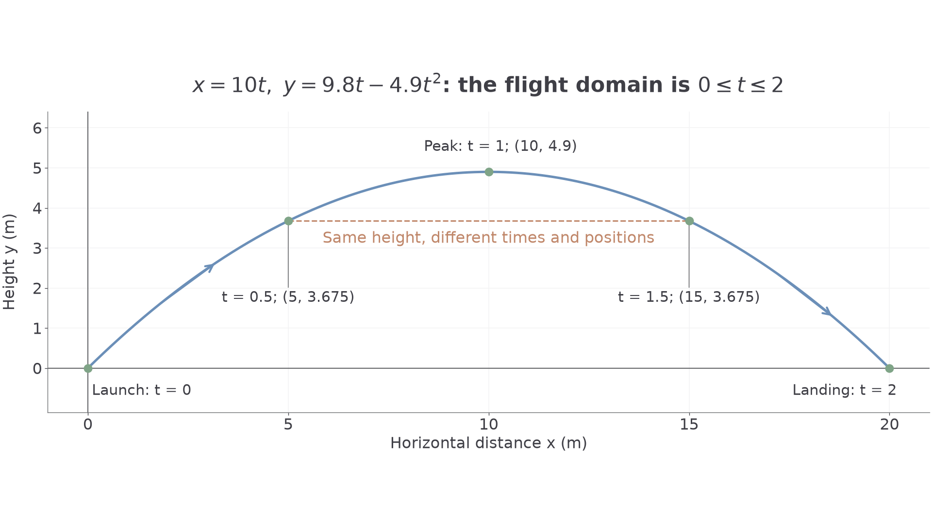
The two marked interior points have the same height but different times and horizontal positions. Equal heights alone cannot identify the location of the object.

Worked example 5: launch from ground level

Question. For $x=10t$ , $y=9.8t-4.9t^2$ , determine the flight domain, Cartesian path and highest point.

Plan. Find ground-level roots, eliminate $t$ and complete the square in height.

\begin{aligned} y&=4.9t(2-t)=0 &&\text{ground level}\\ t&=0\text{ or }2 &&\text{launch or landing}\\ y&=0.98x-0.049x^2,\quad0\le x\le20 &&\text{use }t=x/10\\ y&=4.9-4.9(t-1)^2 &&\text{complete the square} \end{aligned}

Why this step? The zero root is launch; the positive root gives the end of the airborne model.

Answer. $0\le t\le2$ ; the path is the stated restricted parabola. The highest point is $(10,4.9)$ at $t=1$ .

Check. At $t=0.5,1.5$ , height is $3.675\,\mathrm m$ , with horizontal coordinates $5,15\,\mathrm m$ .

Change only the initial height by adding $14.7\,\mathrm m$ . The horizontal motion and quadratic height coefficients remain unchanged.

Worked example 6: launch above ground level

Question. For $x=10t$ , $y=14.7+9.8t-4.9t^2$ , determine the flight domain, Cartesian path and highest point.

Plan. Solve the new ground equation and reject any root before launch.

\begin{aligned} y&=4.9(3+2t-t^2) &&\text{factor out }4.9\\ 0&=(3-t)(t+1) &&\text{ground equation}\\ t&=3\text{ or }-1 &&\text{solve}\\ y&=14.7+0.98x-0.049x^2 &&\text{eliminate time}\\ y&=19.6-4.9(t-1)^2 &&\text{complete the square} \end{aligned}

Why this step? A negative root describes where the extended algebraic path meets ground before the launch time; it is outside the model.

Answer. $0\le t\le3$ , with $0\le x\le30$ . The highest point is $(10,19.6)$ , at $t=1$ .

Check. At $t=3$ , $14.7+29.4-44.1=0$ ; at $t=0$ , the initial height is $14.7$ .

The first flight's average vertical coordinate rate is $4.9\,\mathrm{m\,s^{-1}}$ from launch to peak and $-4.9\,\mathrm{m\,s^{-1}}$ from peak to landing. Its horizontal rate is $10\,\mathrm{m\,s^{-1}}$ . These are interval averages, not a claim of constant vertical motion. The supplied height models and derived Cartesian equations are not formula-sheet results to memorise; use the given model.

Watch out

Wrong: both roots $-1$ and $3$ are possible landing times after launch. Right: apply $t\ge0$ , then stop the model at the first ground contact after launch.

Keep the same model structure and change the initial height again.

Checking a parametric model against observations

Matching a path is weaker than matching a timed journey. A useful model must predict both coordinates at the observation time and explain its assumptions well enough to investigate discrepancies.

Observed minus predicted

A coordinate discrepancy is the observed coordinate minus the model's prediction, using the same axes, time origin and units. Its sign records the direction of the mismatch; it does not identify a unique cause.

For example, the ground-level flight predicts $(10,4.9)$ at $t=1$ . An observation $(10.3,4.6)$ gives discrepancies $(0.3,-0.3)\,\mathrm m$ . Air resistance, launch uncertainty and measurement error are possibilities, rather than conclusions forced by that one observation.

Worked example 7: a boat observation

Question. A boat is modelled by $x=2+1.5t$ , $y=3-0.5t$ , $0\le t\le5$ , in metres and seconds. At $t=4$ , its observed position is $(8.3,1.2)$ . Calculate the discrepancies and state one relevant assumption to investigate.

Plan. Predict both coordinates at the known time, then subtract and interpret.

\begin{aligned} (x,y)_{\text{predicted}}&=(2+1.5(4),\ 3-0.5(4))=(8,1) &&\text{same observation time}\\ \text{observed}-\text{predicted}&=(8.3-8,\ 1.2-1) &&\text{coordinate differences}\\ &=(0.3,0.2)\,\mathrm m &&\text{retain units} \end{aligned}

Why this step? A discrepancy must compare positions at the same time, not simply the nearest point on a drawn path.

Answer. $(0.3,0.2)\,\mathrm m$ . Investigate constant coordinate rates, for example whether steering or the current changed.

Check. Prediction plus discrepancy returns $(8.3,1.2)$ .

Change only the observed position to $(7.8,0.9)$ . The prediction and observation time stay fixed.

Worked example 8: interpret the mismatch cautiously

Question. Calculate the new discrepancies and explain whether they establish that the current changed.

Plan. Reuse the prediction and separate evidence of mismatch from evidence of a cause.

\begin{aligned} (x,y)_{\text{predicted}}&=(8,1) &&\text{unchanged model and time}\\ \text{observed}-\text{predicted}&=(7.8-8,\ 0.9-1) &&\text{subtract}\\ &=(-0.2,-0.1)\,\mathrm m &&\text{signed discrepancy} \end{aligned}

Why this step? Several assumptions and measurement errors could explain a mismatch; one pair of coordinates cannot isolate one of them.

Answer. $(-0.2,-0.1)\,\mathrm m$ . The observation does not establish a changing current; collect observations across the interval and consider measurement uncertainty.

Check. $(8,1)+(-0.2,-0.1)=(7.8,0.9)$ .

There is another subtle check. The model $x=2+3t$ , $y=1+2t$ , $0\le t\le4$ , and $x=2+6s$ , $y=1+4s$ , $0\le s\le2$ , have the same Cartesian path. If $s=t/2$ is a new label, they describe the same journey. If both parameters mean actual seconds after departure, the second journey is twice as fast along that segment: at one second the positions are $(5,3)$ and $(8,5)$ . Timing survives in the parametric model but disappears on elimination. This comparison is not a formula-sheet result.

Key idea

Evaluate a model using its domain, timing and assumptions as well as its curve. A good algebraic fit does not by itself validate the physical interpretation.

Try a fresh observation of the same boat.

Quick Recap

State the parameter's meaning, units and physical domain.
A changed parameter definition needs changed equations and a translated domain.
A time model retains timing information that its Cartesian path loses.
Ground roots before launch and heights after landing are outside the airborne model.
Compare observations at the stated time, then investigate assumptions without inferring a unique cause from one mismatch.

The opening question is resolved by the domain: a zero-width rectangle and a post-landing flight point may satisfy equations, but neither belongs to the physical situation being modelled.

Last Accessed

Pure Mathematics

Statistics

Mechanics

Mg16 - Parametric models and restricted parameters

Constructing a model with a shared parameter

Time, position and average changes

A projectile path with a physical domain

Checking a parametric model against observations

Quick Recap

Learn faster with Nova