Mc34, Mc35 - Trapezium rule and area bounds | OCR A-Level Mathematics B (MEI)

Could a zero estimate hide a positive area? Under Mc34, you will construct and interpret trapezium estimates and justify their error direction on an interval of consistent concavity. Under Mc35, you will use rectangle sums for bounds, then read an unfamiliar expression for the same trapezium method.

Build the composite trapezium rule

The curve $16x^2(1-x)^2$ has height zero at both ends of $[0,1]$ , so a single trapezium gives zero. Yet the curve is positive inside and its exact integral is $8/15$ . Sampling can miss an entire hill!

You already know

A trapezium of width $h$ and parallel heights $p,q$ contributes $h(p+q)/2$ . Definite integrals are signed; geometric area needs magnitudes if the curve crosses the axis.

Use $n$ equal strips of width $h=(b-a)/n$ . There are $n+1$ ordinates $y_i=f(a+ih)$ , including both endpoints.

Trapezium rule

For equally spaced ordinates,

T_n=\frac h2[y_0+2(y_1+\cdots+y_{n-1})+y_n] \approx\int_a^b f(x)\,\mathrm dx.

In the formula sheet.

Every interior ordinate belongs to two adjacent strips, explaining its weight $2$ .

Worked example 1: applying the weights

Question. Estimate $\int_0^1\mathrm e^x\,\mathrm dx$ with two equal strips.

Plan. Calculate three heights, then form the weighted sum.

\begin{aligned} h&=\frac12,\qquad (y_0,y_1,y_2)=(1,\mathrm e^{1/2},\mathrm e)\\ T_2&=\frac14[1+2\mathrm e^{1/2}+\mathrm e]\\ &=1.753931092\ldots \end{aligned}

Why three heights? Two strips share the middle ordinate but each needs two boundary heights.

Answer. The estimate is $1.75393$ to five decimal places.

Check. The exact integral is $\mathrm e-1\approx1.71828$ , so this is an overestimate.

Change only the strip count to four.

Worked example 2: more strips

Question. Estimate the same integral using four equal strips.

Plan. Insert the quarter-step heights and retain their full values.

\begin{aligned} h&=\frac14\\ T_4&=\frac18[1+2(\mathrm e^{1/4}+\mathrm e^{1/2}+\mathrm e^{3/4})+\mathrm e]\\ &=1.727221905\ldots \end{aligned}

Why retain the middle height? Refining adds ordinates; it does not discard those already sampled.

Answer. The estimate is $1.72722$ to five decimal places.

Check. It is closer to $\mathrm e-1$ than the two-strip estimate.

For the polynomial $x^2+1$ on $[0,2]$ , five heights $1,1.25,2,3.25,5$ give $T_4=4.75$ ; the individual trapezia $0.5625,0.8125,1.3125,2.0625$ give the same total. Another table, $2,3,6,11$ at $0,1,2,3$ , gives $15.5$ .

Exam tip

If instructed to use the trapezium rule, show a substituted expression with every ordinate. “Determine” requires justified working, and four strips require five heights.

Refine the exponential example once more.

Use technology and refine the estimate

For $\mathrm e^{-x^2}$ , elementary antiderivatives do not supply a formula, so a calculator table is especially useful. A spreadsheet can store inputs, ordinates, weights and weighted values; use full stored precision and round only the final total.

Worked example 3: a table without an elementary antiderivative

Question. Estimate $\int_0^1\mathrm e^{-x^2}\,\mathrm dx$ with two equal strips.

Plan. Evaluate the function at $0,0.5,1$ , then apply endpoint/interior weights.

\begin{aligned} (y_0,y_1,y_2)&=(1,\mathrm e^{-1/4},\mathrm e^{-1})\\ T_2&=\frac14[1+2\mathrm e^{-1/4}+\mathrm e^{-1}]\\ &=0.731370252\ldots \end{aligned}

Why evaluate the function, rather than use the inputs as heights? The inputs give strip positions; the outputs supply areas.

Answer. $T_2\approx0.731370$ .

Check. Adding the two individual trapezia gives the same total.

Change only the strip count to four.

Worked example 4: refining the table

Question. Repeat with four equal strips.

Plan. Add values at $0.25$ and $0.75$ without rounding the stored ordinates.

\begin{aligned} T_4&=\frac18[1+2(\mathrm e^{-1/16}+\mathrm e^{-1/4}+\mathrm e^{-9/16})+\mathrm e^{-1}]\\ &=0.742984098\ldots \end{aligned}

Why does the changed answer not alone give an error bound? It compares two approximations; neither has yet been proved to enclose the integral.

Answer. $T_4\approx0.742984$ .

Check. Eight strips give $0.745865615\ldots$ , showing further movement rather than exact agreement.

For unequal spacings, use separate widths. Readings $(0,4),(1,6),(3,2)$ give $\frac12(4+6)(1)+\frac12(6+2)(2)=13$ . A common-width formula is invalid there. Do not invent new measured heights when refining a sparse data table: take more readings or state an interpolation assumption.

Watch out

More printed digits do not mean more reliable data. A narrow peak between sampled inputs can remain hidden, as the opening zero-height example shows.

Keep the same Gaussian function and refine once more.

Decide the direction of trapezium error

The curve's concavity determines which side of each chord it lies on. Increasing or decreasing behaviour alone does not decide trapezium bias.

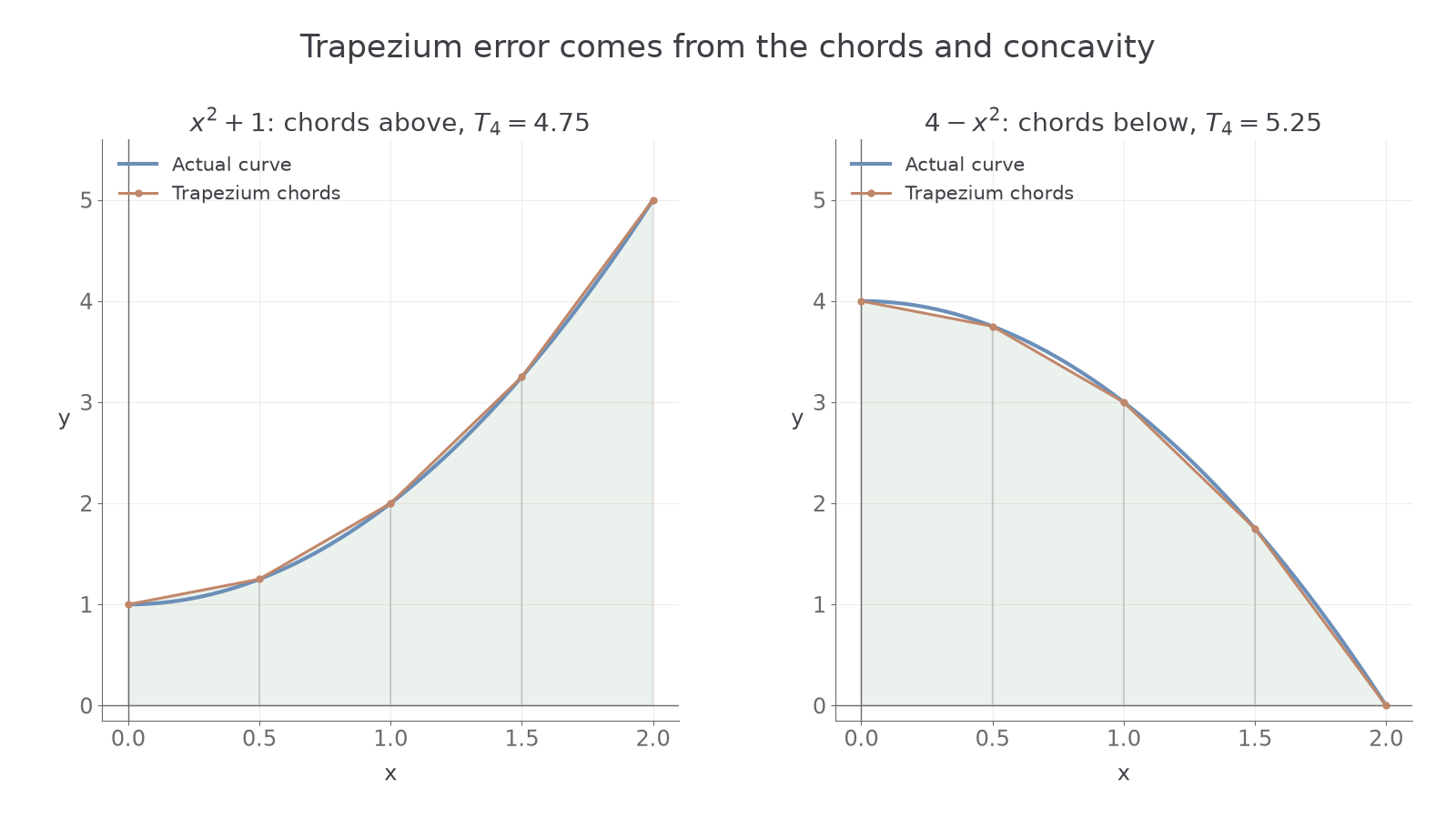
Trapezium chords above and below curves

The diagram shows $x^2+1$ , whose chords lie above it, and $4-x^2$ , whose chords lie below it. Four strips give $4.75>14/3$ and $5.25<16/3$ , respectively.

Concavity and the error direction

On an interval of consistent concavity:

\begin{aligned} f''(x)\ge0&\Rightarrow T_n\ge I && \text{concave upwards}\\ f''(x)\le0&\Rightarrow T_n\le I && \text{concave downwards} \end{aligned}

where $I=\int_a^b f(x)\,\mathrm dx$ . The chords lie above the curve in the first case and below in the second.

Not in the formula sheet: learn it.

Use an interval-wide reason, then state “overestimate” or “underestimate” explicitly.

Worked example 5: consistent upward concavity

Question. Decide the trapezium error direction for $f(x)=2+1/(1+x)$ on $[0,2]$ .

Plan. Differentiate twice and inspect the sign.

f''(x)=\frac{2}{(1+x)^3}>0\qquad(0\le x\le2).

Why check the whole interval? One positive second derivative at a single point does not establish consistent concavity.

Answer. The curve is concave upwards, its chords lie above it, and the integral is overestimated.

Check. The denominator is positive everywhere in the interval; there is no excluded point.

Change only the sign of the reciprocal term.

Worked example 6: reversing concavity

Question. Decide the error direction for $f(x)=2-1/(1+x)$ on the same interval.

Plan. Reverse the sign of the second derivative.

f''(x)=-\frac{2}{(1+x)^3}<0.

Why does the chord position reverse? Reflecting the varying term reverses the direction of curvature.

Answer. The curve is concave downwards; chords lie below it, giving an underestimate.

Check. Both functions remain positive here, so the signed-integral comparison also describes their geometric areas.

Continue this lesson.

You’re previewing NovaLearn without an account. Create a free account to read the rest.

Create free account

Last Accessed

Pure Mathematics

Statistics

Mechanics

Mc34, Mc35 - Trapezium rule and area bounds

Build the composite trapezium rule

Use technology and refine the estimate

Decide the direction of trapezium error

Continue this lesson.

Learn faster with Nova