2b, 2c - Exploring the 2027 large data set

LDS9 is a historical sample of people

Why does a person with systolic readings $104$, $104$ and $112$ have a supplied average of $108$, rather than $106.7$? The answer is in the measurement rule, not a mysterious new way to add. This is the first real person in the workbook, and the rule will matter whenever you analyse its blood-pressure columns.

For the H640 June $2027$ examination, the prescribed resource is LDS9, with its student notes and source information. It contains a random sample of $200$ people aged $16$ or over from the American National Health and Nutrition Examination Survey, NHANES, in $2003$–$2004$. Read the Information sheet. These public-domain survey data were downloaded for the resource in $2017$. LDS10 belongs to later H640 examinations, not June $2027$.

One Data row is one person. Age is in years; Weight is in kg; Height, waist and limb lengths are in cm; Pulse counts beats over $60$ seconds; blood pressures are in mmHg. Sex, Marital, Food30 and Arm are categorical fields. Marital categories have no numerical rank that would justify calculating a correlation from arbitrary category numbers.

For example, the first person's mass $60.3\,\mathrm{kg}$ and height $173.4\,\mathrm{cm}=1.734\,\mathrm m$ give BMI $60.3/1.734^2=20.0548\ldots$, agreeing with the supplied $20.05$. BMI uses mass in kg divided by squared height in metres; the centimetre value must be converted. This definition is supplied by the context, not printed in the formula sheet.

For blood pressure, interviewers sought three measurements at least one minute apart, with at most four attempts. The supplied Systolic and Diastolic averages ignore the first reading unless it is the only reading. Here “first reading” means the first successfully recorded measurement: if attempt one is missing, it is not necessarily the first column. Average the remaining recorded readings, not missing attempts. The Data headers misspell the individual diastolic fields as “Disatolic1” to “Disatolic4”; retain those labels when locating source columns, while writing “diastolic” in your conclusions.

Change only the person in Worked example 2. The measurement protocol and missing-fourth-attempt pattern stay the same.

If only the first reading exists, retain it instead: discarding it would discard the person's only measurement. No blood-pressure averaging protocol or arithmetic-mean formula is printed in the formula sheet; learn to apply the supplied definition.

A third real row gives you the same calculation without copying either example.

Complete observations are selected for named variables

Choose the variables before removing unavailable values; a person with a missing arm length can still contribute to an age–blood-pressure enquiry.

Keep the source unchanged. In a working copy, retain the original Data row number as an identifier, and select Age with the measurement you need. A spreadsheet column holds a field, a row holds a person's observations, and a cell such as U2 identifies a particular entry. Delete or exclude a whole selected analysis row when a required member of its pair is missing; never shift individual cells upward, which would pair different people.

For Age against Systolic, original columns B and U must both be numeric. All $200$ ages are present, but $14$ Systolic values are missing, leaving $186$ complete pairs. A missing fourth attempt does not invalidate an available supplied average. Compact the selected pairs into a separate analysis table: merely hiding rows does not make ordinary spreadsheet summary functions ignore them.

On a compact table with row $1$ containing headers and the selected measurement in column C, use $\texttt{COUNT}$, $\texttt{AVERAGE}$ and $\texttt{STDEV.S}$ on the explicit data range. The letter S in this function is a useful reminder of the sample divisor; check your calculator's output definition rather than guessing from its label.

Change only the blood-pressure variable to Diastolic. Its own data quality determines its selected count; do not carry over the earlier count automatically.

The original first complete Age–Systolic pairs are useful spot checks on copying:

Record your variables, excluded codes or errors, final count and units. A tidy table does not establish representativeness: missingness may relate to health or measurement difficulty.

For a fresh summary, keep Age and change the measured variable to Pulse.

Software graphs and outputs explore relationships

An XY scatter diagram puts one person at each complete Age–Systolic pair, so the horizontal and vertical coordinates must stay together.

Select the two columns in the compact $186$-pair table and insert an XY scatter chart, with Age horizontally and Systolic vertically. Label years and mmHg. Do not use a line chart joining people in workbook order: that order is not elapsed time. A point can coincide with another person's point, so fewer visible dots need not mean fewer observations.

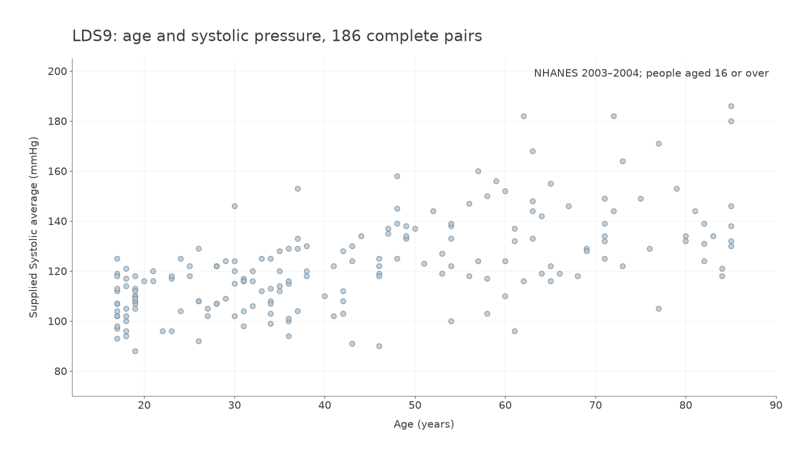
The pattern suggests positive association with considerable variation. On the compact table, $\texttt{=CORREL(B2:B187,C2:C187)}$ gives approximately $0.616$. This describes linear association in these pairs. It is neither a slope nor a claim that $61.6\%$ of people have a particular condition. Calculating this coefficient by hand is unnecessary here.

For group comparisons, create separate Sex-group scatter plots with common scales. The available female Systolic values have count $94$, mean $123.798$ and sample SD $22.508\,\mathrm{mmHg}$; the male values have count $92$, mean $121.109$ and sample SD $14.397\,\mathrm{mmHg}$. The observed female spread is greater, but differences in age composition and missingness may affect the comparison. Use a box plot for median and IQR, a histogram for shape, and a bar chart for categorical counts such as Marital.

Choose a numerical threshold as a mathematical event, without turning it into a diagnosis. Count the event and its eligible total using the same cleaned range. The frequency-over-total reasoning is not printed as a separate formula in the formula sheet: learn it.