MH1–MH3 - Hypotheses, significance and statistical decisions
Can a sample distinguish a real improvement from ordinary variation? Use a binomial model to set population hypotheses, choose one or two tails, and interpret a significance test as evidence with a controlled risk of a wrong decision.
The null model concerns a population probability
Would seven replies from twelve independent invitations be convincing evidence that a response probability has increased from ? First decide which population claim the sample is meant to investigate.
You already know
A binomial count needs a fixed number of independent trials, two outcomes and a common success probability. Write ; is random, while an observed count is one realised value.
Calling a reply a “success” is simply a mathematical label. It does not imply that replying is better than not replying.
Population hypotheses
The null hypothesis, , is the default population claim. The alternative hypothesis, , describes the departure being investigated. A hypothesis about a probability concerns the whole population, not the observed sample proportion.
The null fixes a model from which we calculate the probabilities of possible samples. A small sample cannot tell us the population probability exactly.
Worked example 1: specifying an improvement
Question. A response probability is claimed to be . Investigate whether it has increased, using twelve independent invitations. State the hypotheses and null distribution.
Plan. Define the probability in context and translate “increased”.
Why this step? The count model uses the probability claimed by the null, not the sample proportion observed later.
Answer. This is an upper one-tail test. The test statistic is the random number of replies.
Check. If seven reply, is the observation. It is not a hypothesis about .
Keep the sampling experiment fixed and change only the question to “has the probability changed?”
Worked example 2: allowing either direction
Question. State the hypotheses and tail choice when any change from the claimed response probability is of interest.
Plan. Keep the equality in the null and allow both departures.
Why this step? “Changed” includes a decrease as well as an increase, even if the eventual sample happens to have many replies.
Answer. This is a two-tail test about the population reply probability.
Check. The null distribution stays the same. The alternative changes which outcomes count as extreme evidence.
A lower one-tail test would instead use . The question fixes the choice before inspecting the count.
Watch out
Choosing the favourable tail after seeing the data changes the procedure's error risk. A sample above the claim does not justify replacing a planned two-tail test with an upper-tail test.
Set up a new investigation without calculating a tail yet.
Extreme events determine a test decision
A large reply count is evidence for an increase only if that count, or something still more extreme, is sufficiently unlikely under the null.
p-value
The p-value is the probability, under the null hypothesis and sampling model, of an outcome at least as extreme as the observation in the direction of the alternative.
For an upper-tail test, an observed seven replies contributes , not just . Choose a significance level before sampling and reject when the directed p-value is at most . The hypothesis-testing definitions and this decision rule are not in the formula sheet: learn their meaning.
Critical region and acceptance region
The critical region, or rejection region, contains the values of the test statistic leading to rejection. Its boundary is a critical value. The other possible values form the acceptance region: the region for which the test does not reject the null, rather than prove it.
The probability route and the critical-region route express the same decision. Seeing them side by side makes the boundary meaningful.
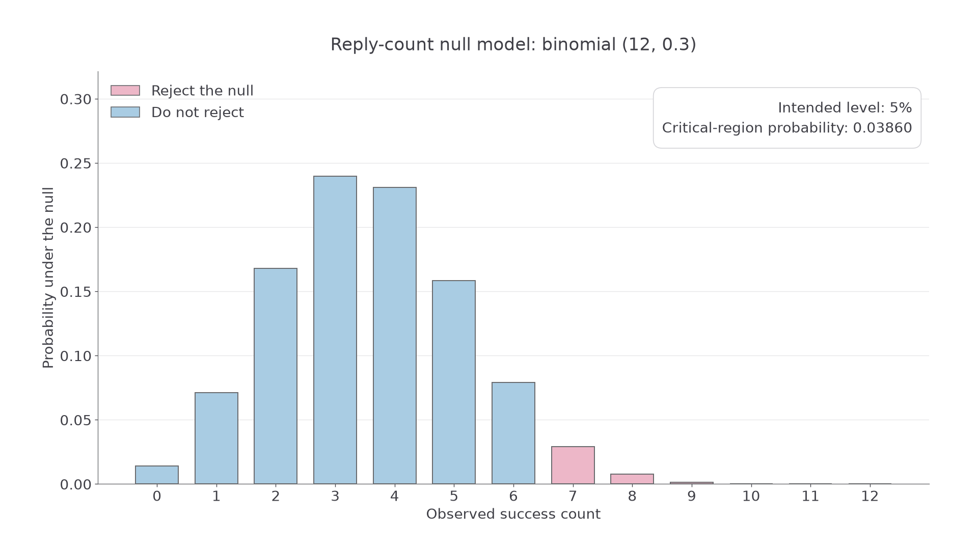
At the level, six replies are outside the critical region; seven are inside it.
Continue this lesson.
You’re previewing NovaLearn without an account. Create a free account to read the rest.
Create free account