MR1–MR5 - Binomial models and probabilities

Define the count and test the trial conditions

A team contacts five people at a time. If each replies with probability 0.4, should most batches contain exactly two replies? The average count and the most common count can agree without either occurring in most batches. A probability model will tell us the difference.

Fix a deadline and count replies by that deadline. A person's eventual reply is a different event and may have a different probability.

For five contacts, a common reply probability 0.4 and independent replies give $X\sim\mathrm B(5,0.4)$. The fixed five contacts and reply/no-reply deadline rule establish two conditions. Common probability and independence are assumptions to assess against the context.

Different levels of familiarity with the team could change $p$ between people. Members of one household could discuss the message, linking their replies. Those are different objections: unequal probabilities and dependence. Stopping when the first reply arrives would instead remove the fixed trial number. Sampling without replacement from a small known group of responders and non-responders generally changes the success proportion as selections proceed.

Observed data can suggest $p$. For example, 48 replies from 120 earlier contacts give estimated reply probability $48/120=0.4$. Applying that to a new group assumes comparable people, message and deadline; the estimate does not make 0.4 an exact known population probability.

For a different setting, the 2027 MEI large data set contains 200 NHANES records from people aged 16 or over in the 2003–04 survey. Imagine drawing five records without replacement and counting those aged at least 40. The age threshold gives a binary classification, but selecting a record changes the mix remaining, so the count is generally not exactly binomial. A model for random draws from these records also concerns this historical finite data set; it does not automatically describe people in the United States today.

Consider what is still missing when the trial number and success probability are already specified.

Calculate the probability of an exact count

The count two hides several possible reply lists. A combination factor counts every choice of the two people who reply.

One specified list has product probability $p^rq^{n-r}$ by independence. Constant $p$ makes this probability the same for all $\binom nr$ disjoint lists. Their sum gives the formula. Equivalently, all count probabilities appear as the terms of $(q+p)^n=1$.

Change only the required count, from two replies to three. The number of contacts and reply probability stay fixed.

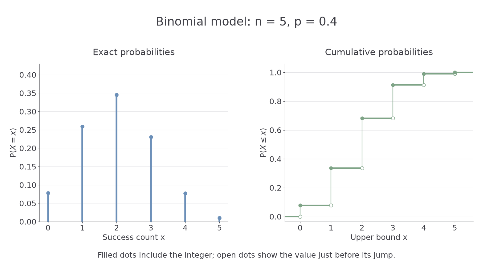
A calculator's exact binomial function needs $n,p,r$, although the entry order depends on the device. Distinguish it from cumulative output. The endpoint check $\mathrm P(X=0)=0.6^5=0.07776$ is especially useful; $\mathrm P(X=5)=0.4^5=0.01024$. Impossible counts have probability zero. When $p=0$ or $p=1$, the count is certain, respectively 0 or $n$.

Keep unrounded values for further work. Use a stated accuracy in the answer; the following question explicitly requests three significant figures.

Use the correct integer boundary for a tail

A cumulative function adds whole probability spikes, including the integer used as its endpoint.