Ma14 - Proportional relationships and models | OCR A-Level Mathematics B (MEI)

A proportional relationship might be a line, a reciprocal curve or a root curve. Learn to identify what stays constant, build the equation and use both observations and graph labels to judge a model.

Direct proportion and its constant

A pump fills a tank in $80$ seconds at $3$ litres per second. Would twice the rate mean twice the time? Before calculating, imagine the same water arriving twice as quickly. The answer should go the other way. We will return to that prediction after separating direct from inverse proportion.

You already know

An equation can contain a fixed parameter and a changing input. Substitute one known pair to determine a parameter; use a different pair to test the resulting model.

A fixed price per litre gives a simpler starting point: the amount paid is a constant multiple of the volume bought.

Direct proportion

$y\propto x$ means $y=kx$ for a constant $k$ on the stated domain. The ratio $y/x$ is constant when $x\ne0$ . A line such as $y=2x$ is an example; $y=2x+7$ is not, because its nonzero intercept changes the ratio.

The full graph is a line through the origin, with gradient $k$ . A context may allow only its non-negative portion. The units of $k$ are output units divided by input units: pounds per litre, for example.

Calibrating direct proportion

y=kx,\qquad k=\frac{y}{x}\quad(x\ne0)

Use the same constant for all permitted inputs.

Not in the formula sheet: learn it.

“Determine” asks you to justify the result. One clear substitution followed by the new prediction makes that route visible.

Worked example 1: a constant price

Question. The cost $C$ pounds is directly proportional to the volume $V$ litres. Given $C=20$ at $V=8$ , determine the equation and the cost of $14$ litres.

Plan. Divide cost by volume to find the fixed price, then use it for the new volume.

\begin{aligned} k&=\frac{20}{8}=\frac52 &&\text{calibrate in pounds per litre}\\ C&=\frac52V &&\text{write the model}\\ C(14)&=\frac52(14)=35 &&\text{substitute the new volume} \end{aligned}

Why this step? The relationship is assumed proportional, so the price per litre is the same at both volumes.

Answer. $C=2.5V$ ; $14$ litres costs $35$ pounds.

Check. $35/14=20/8=2.5$ pounds per litre.

Now change only the calibration cost, representing a different fixed price. The method and requested volume stay the same.

Worked example 2: recalibrating the price

Question. $C$ pounds is directly proportional to $V$ litres. Given $C=24$ at $V=8$ , determine the equation and the cost of $14$ litres.

Plan. Find the new constant before using the new input.

\begin{aligned} k&=\frac{24}{8}=3 &&\text{new price per litre}\\ C&=3V &&\text{insert the constant}\\ C(14)&=3(14)=42 &&\text{evaluate} \end{aligned}

Why this step? A new calibration defines a new model; the constant from the previous example does not belong to it.

Answer. $C=3V$ ; the cost is $42$ pounds.

Check. The volume multiplier is $14/8$ , and $24(14/8)=42$ .

Positive examples are familiar, but the mathematical definition also allows a negative constant and a line sloping down through the origin.

Watch out

Wrong: “Both quantities increase, so they are directly proportional.” Right: establish a constant ratio. For $y=2x+7$ , both increase for positive $x$ , but $y/x=2+7/x$ changes.

Keep the cost-volume setting and try a new calibration.

Proportion to a power or root

In $y\propto x^2$ , it is $x^2$ , rather than $x$ , that is multiplied by a constant. This small change explains why a proportional graph can curve.

Scale a cube so that every length doubles. Each face now has four times the area, while the cube holds eight times the volume. The larger cube therefore has half as much surface area per unit volume: $4/8=1/2$ . A single size multiplier can have very different effects.

Power and root variation

For permitted positive inputs,

y=kx^n\quad\Longrightarrow\quad \frac{y_2}{y_1}=\left(\frac{x_2}{x_1}\right)^n

The ratio form requires $k\ne0$ . A square root uses $n=1/2$ ; a cube root uses $n=1/3$ . Check the real domain: square roots allow non-negative arguments, while cube roots also allow negative arguments if the context permits them.

Not in the formula sheet: learn it.

To calibrate, divide by the entire power or root. Do that operation before applying the model to another input.

Worked example 3: a square model

Question. $y$ is directly proportional to $x^2$ for $x>0$ . Given $y=12$ at $x=4$ , determine $y$ at $x=9$ .

Plan. Find $y/x^2$ , then multiply the new square by that constant.

\begin{aligned} k&=\frac{12}{4^2}=\frac34 &&\text{divide by the square}\\ y&=\frac34(9^2) &&\text{substitute }x=9\\ &=\frac{243}{4} &&\text{simplify exactly} \end{aligned}

Why this step? Dividing by $4$ instead would fit direct proportion to $x$ , a different relationship.

Answer. $y=243/4$ .

Check. $12(9/4)^2=243/4$ ; the output grows faster than the input.

Change only the exponent, replacing the square by a square root. Keeping the same pair and target input isolates that change.

Worked example 4: a root model

Question. $y$ is directly proportional to $\sqrt{x}$ for $x>0$ . Given $y=12$ at $x=4$ , determine $y$ at $x=9$ .

Plan. Calibrate using the old root and evaluate using the new root.

\begin{aligned} k&=\frac{12}{\sqrt4}=6 &&\text{divide by the old root}\\ y&=6\sqrt9 &&\text{use the new input}\\ &=18 &&\text{evaluate the root} \end{aligned}

Why this step? The input multiplier is $9/4$ , but the output multiplier is only $\sqrt{9/4}=3/2$ .

Answer. $y=18$ .

Check. $12/\sqrt4=18/\sqrt9=6$ .

The four-panel picture shows why naming the axes matters. Each panel has its own vertical scale.

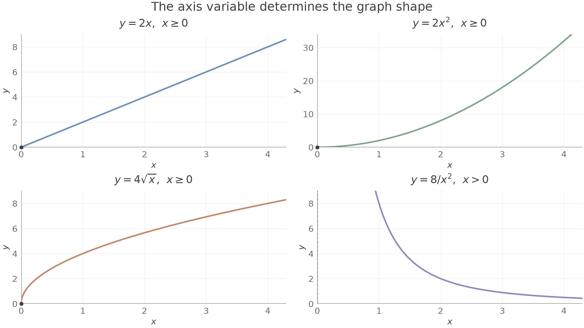
Four direct and inverse proportional relationships on their stated domains

The panels show $y=2x$ , $y=2x^2$ , $y=4\sqrt{x}$ and $y=8/x^2$ . The first three use $x\ge0$ ; the last uses $x>0$ . If the horizontal coordinate were $x^2$ , the square model would instead be a line through the origin. Its gradient would be $k$ , not the gradient of the curve on ordinary $x$ -axes. Plotting against $\sqrt{x}$ does the same for the root model.

Watch out

Wrong: $y\propto\sqrt{x}$ gives $y^2=k\sqrt{x}$ . Right: first write $y=k\sqrt{x}$ . Only then rearrange if a question needs a different form.

A cube-root relationship follows the same method with a different fractional power.

Inverse proportion to powers and roots

Inverse proportion keeps a product constant. The input expression now sits beneath the fraction line.

Inverse proportion

$y$ is inversely proportional to $u$ when $y=k/u$ , equivalently $yu=k$ , for a fixed constant $k$ and $u\ne0$ . For inverse proportion to $x^2$ , the constant product is $yx^2$ , not $yx$ .

For a positive quantity with a positive constant, a larger denominator gives a smaller output. The exponent tells you how much smaller.

Inverse powers and roots

For $x>0$ ,

y=\frac{k}{x^n},\qquad \frac{y_2}{y_1}=\left(\frac{x_2}{x_1}\right)^{-n}

The ratio form requires $k\ne0$ . Inverse-square uses $n=2$ ; inverse-square-root uses $n=1/2$ . The zero input is excluded, and a real square root in a denominator must be strictly positive.

Not in the formula sheet: learn it.

Multiplying by the known denominator isolates $k$ . This is the reverse of the calibration step for direct proportion.

Worked example 5: inverse proportion to a square

Question. $R$ is inversely proportional to $s^2$ , for $s>0$ . Given $R=6$ at $s=4$ , determine $R$ at $s=9$ .

Plan. Find $Rs^2$ , then divide it by the new square.

\begin{aligned} k&=6(4^2)=96 &&\text{calibrate the constant product}\\ R(9)&=\frac{96}{9^2} &&\text{substitute}\\ &=\frac{32}{27} &&\text{simplify} \end{aligned}

Why this step? The denominator grows by $(9/4)^2$ , so the output is divided by that factor.

Answer. $R=32/27$ .

Check. $(32/27)(81)=96=6(16)$ .

Change only the denominator power from $2$ to $1/2$ . The same two input values make a gentler decrease.

Worked example 6: inverse proportion to a root

Question. $R$ is inversely proportional to $\sqrt{s}$ , for $s>0$ . Given $R=6$ at $s=4$ , determine $R$ at $s=9$ .

Plan. Find $R\sqrt{s}$ , then divide by the new root.

\begin{aligned} k&=6\sqrt4=12 &&\text{calibrate}\\ R(9)&=\frac{12}{\sqrt9} &&\text{evaluate at the new input}\\ &=4 &&\text{divide by }3 \end{aligned}

Why this step? Multiplication by $\sqrt{s}$ , rather than $s^2$ , is what leaves the new constant unchanged.

Answer. $R=4$ .

Check. $6\sqrt4=4\sqrt9=12$ .

For nonzero $k$ , reciprocal and inverse-square curves have asymptotes $x=0$ and $y=0$ . Their positive branches never reach zero. A graph of $R$ against $1/\sqrt{s}$ linearises the inverse-root model, giving gradient $k$ ; the horizontal-axis variable already contains the reciprocal.

Watch out

Wrong: “The curve decreases, so it is inverse proportion.” Right: check the specified constant product. Many decreasing curves do not have $xy$ , $x^2y$ or another proposed product constant.

Test both the prediction and the choice of axes in this new case.

Construct and evaluate a proportional model

A proportional model is a claim about a situation, so a convincing answer connects the constant to something that really stays fixed.

For filling a fixed empty tank with no leaks, the product of actual steady flow rate and time is the volume. A single pair sets the constant, but cannot test the assumption. For a data check, compare the appropriate invariant: $y/x$ , $y/x^2$ , $xy$ or $x^2y$ . The pairs $(1,6)$ , $(2,24)$ , $(3,54)$ have $y/x^2=6$ , supporting a square relationship at the observed inputs. That does not prove it beyond them.

Worked example 7: interpreting the constant

Question. A tank takes $80$ seconds to fill at a steady $3$ litres per second. Assume time $T$ is inversely proportional to rate $q$ . Determine the model and compare its prediction at $q=6$ with a measured time of $40$ seconds.

Plan. Calibrate $Tq$ , identify its units and use a separate rate to test the prediction.

\begin{aligned} k&=80(3)=240 &&\text{volume in litres}\\ T&=\frac{240}{q} &&\text{inverse-rate model}\\ T(6)&=40 &&\text{evaluate the prediction} \end{aligned}

Why this step? Seconds multiplied by litres per second gives litres, explaining the physical meaning of the constant.

Answer. $T=240/q$ , for $q>0$ . The measured $40$ seconds agrees with the model.

Check. The rate doubles and the time halves: $6(40)=3(80)=240$ .

Change only the second observed time. Holding the calibrated equation fixed exposes disagreement instead of explaining it away.

Worked example 8: interpreting a discrepancy

Question. A tank takes $80$ seconds at a steady $3$ litres per second. Assume $T\propto1/q$ . Determine the model and compare its prediction at $q=6$ with a measured time of $44$ seconds.

Plan. Use the first pair for calibration and the second pair solely for comparison.

\begin{aligned} T&=\frac{80(3)}q=\frac{240}q &&\text{calibrate}\\ T(6)&=40 &&\text{predict}\\ 44-40&=4 &&\text{measurement minus prediction} \end{aligned}

Why this step? The measured product $6(44)=264$ litres differs from the calibrated $240$ litres; one constant cannot fit both pairs exactly.

Answer. The measurement is $4$ seconds above the prediction. A startup delay or a flow rate that is not steady could contribute; the figures alone do not establish the cause.

Check. Both times are positive and the prediction has the expected decreasing behaviour. The model cannot include $q=0$ .

The opening question is settled: twice the actual steady rate gives half the time when the volume remains fixed. Very large quoted rates need care, because equipment capacity can prevent them being maintained.

Exam tip

A request to comment on suitability needs a contextual reason. Name what is assumed fixed, or what could change; agreement with one observation is evidence rather than proof of the model.

Apply that distinction to a machine working through a fixed batch.

Quick Recap

Identify the constant ratio or product before calculating.
Direct and inverse proportion can involve a power or a root of the input.
The horizontal-axis variable determines whether a proportional model looks linear.
Calibrate with one observation, then test with another, respecting the model's domain and assumptions.

Twice the tank's steady flow gives half the filling time: $80$ seconds becomes $40$ seconds under the fixed-volume model.

Last Accessed

Pure Mathematics

Statistics

Mechanics

Ma14 - Proportional relationships and models

Direct proportion and its constant

Proportion to a power or root

Inverse proportion to powers and roots

Construct and evaluate a proportional model

Quick Recap

Learn faster with Nova