Mg7 - Straight line models and rates of change | OCR A-Level Mathematics B (MEI)

Construct and question straight-line models in practical settings. You will explain the assumptions behind constant rates, interpret parameters with units, change the input origin and decide what new observations say about a model.

Constant change and model assumptions

A reservoir contains $360$ litres at the first reading and $270$ litres six minutes later. When will it be empty? A straight line offers an answer, but the key mathematical choice comes before the calculation: assume that water continues to leave at a constant net rate.

You already know

In $y=mx+c$ , $m$ measures output change per unit input change. The value $c$ is the output at the chosen input zero, which may lie outside the observed range.

Modelling means making a useful representation and knowing what you have assumed. A fixed unit price can give an exact linear rule within its stated conditions; measured quantities rarely follow a line perfectly.

Straight-line model

A straight-line model uses a relationship such as $Y=mx+c$ , with a constant rate $m$ . State what both variables mean, their units, the allowed inputs and the assumptions under which the rule is intended to apply.

Equal input increments then give equal output increments. That is a stronger claim than merely knowing two points.

Worked example 1: identifying the two charges

Question. An art workshop charges £ $18$ setup plus £ $0.60$ per printed card, for at most $50$ cards. Even a booking for no cards incurs the setup fee. Construct and interpret its cost model.

Plan. Add the fixed charge to the rate multiplied by the number of cards.

\begin{aligned} \text{printing charge}&=0.60n && \text{rate times count} \\ C&=18+0.60n && \text{include the setup} \\ C(10)&=24 && \text{evaluate a booking} \end{aligned}

Why restrict the inputs to integers? Cards are counted, rather than measured continuously.

Answer. $C$ is pounds and $n$ is an integer with $0\le n\le50$ . The intercept is the £ $18$ setup; the gradient is £ $0.60$ per card. The rule assumes no discount or additional charge in this range.

Check. $C(11)=24.60$ , exactly £ $0.60$ more than $C(10)$ .

Remove only the setup charge. Keep the same per-card rate and allowed inputs.

Worked example 2: removing the fixed part

Question. The workshop offers the same printing at £ $0.60$ per card with no setup fee. Give the new model and compare a ten-card booking.

Plan. Set the fixed term to zero, leaving the rate unchanged.

\begin{aligned} C&=0.60n && \text{no fixed charge} \\ C(10)&=6 && \text{ten cards} \\ 24-6&=18 && \text{compare the two tariffs} \end{aligned}

Why is the saving independent of the card count? Only the fixed term was removed.

Answer. $C=0.60n$ , with integer $0\le n\le50$ . Ten cards cost £ $6$ , a saving of £ $18$ .

Check. At $n=20$ , the prices are £ $30$ and £ $12$ , again differing by £ $18$ .

A line with a nonzero fixed term is not direct proportion: the first tariff gives $C(20)=30$ , while $2C(10)=48$ . The contextual cost formulas are not in the formula sheet; form them from the stated rules.

Watch out

Wrong: a gradient of $0.60$ means the setup costs £ $0.60$ . Right: the gradient is £ $0.60$ per card; the intercept is the setup charge.

Interpret a new rule and identify the assumption that makes a single line reasonable.

Constructing a model from two observations

The reservoir readings suggest a loss of $90$ litres in six minutes. A line treats that as a constant loss of $15$ litres each minute; the observations themselves only establish an average.

Constructing a constant-rate model

From observations $(t_1,V_1)$ , $(t_2,V_2)$ , with different input values,

m=\frac{V_2-V_1}{t_2-t_1},\qquad V-V_1=m(t-t_1)

Choose the variable's zero and the model's domain explicitly.

Not in the formula sheet: learn it.

A physically sensible domain is part of the answer, especially when a decreasing line eventually predicts a negative quantity.

Worked example 3: a reservoir emptying

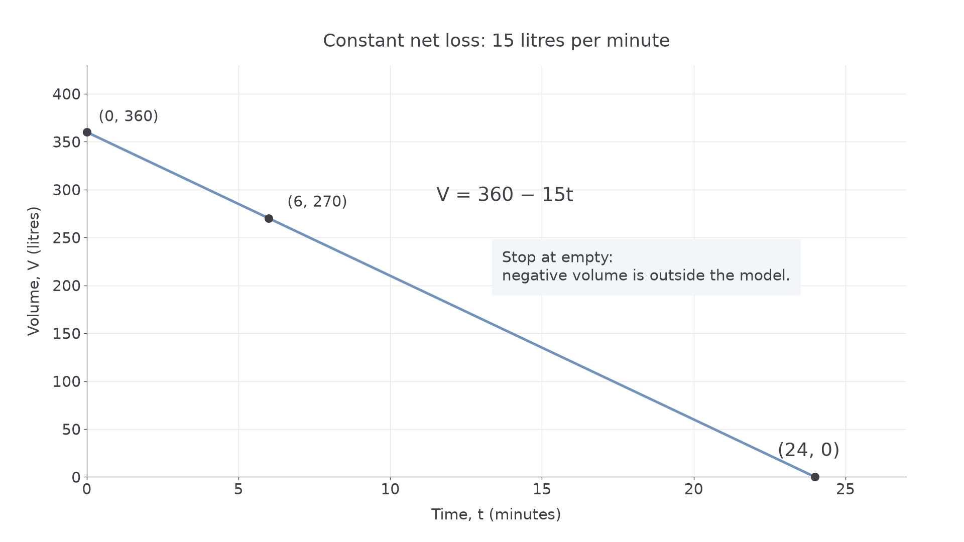
Question. At $t=0$ , a reservoir contains $360$ litres. At $t=6$ minutes, it contains $270$ litres. Assuming a constant net loss, determine the volume model and predicted emptying time.

Plan. Calculate the gradient, use the initial reading and solve for zero volume.

\begin{aligned} m&=\frac{270-360}{6-0}=-15 && \text{litres per minute} \\ V&=360-15t && \text{use }V(0)=360 \\ 360-15t&=0 && \text{set the volume to zero} \\ t&=24 && \text{solve} \end{aligned}

Why stop at zero? Negative volume is outside the physical meaning of this model.

Answer. $V=360-15t$ for $0\le t\le24$ , with emptying predicted after $24$ minutes if the loss remains constant.

Check. $V(6)=270$ , and $V(24)=0$ .

Change only the clock origin. The same readings now occur at $t=2$ and $t=8$ .

Worked example 4: a different clock

Question. The reservoir contains $360$ litres at $t=2$ minutes and $270$ litres at $t=8$ . Under the same constant-loss assumption, determine the model and the clock reading when empty.

Plan. Use the unchanged rate with an observed point to find the intercept.

\begin{aligned} m&=\frac{-90}{6}=-15 && \text{same elapsed interval} \\ V-360&=-15(t-2) && \text{use the first reading} \\ V&=390-15t && \text{expand} \\ 390-15t=0&\Rightarrow t=26 && \text{solve for emptying} \end{aligned}

Why is $360$ not the intercept? That volume belongs to $t=2$ , rather than the chosen zero.

Answer. $V=390-15t$ , with predicted emptying at clock reading $26$ minutes, still $24$ minutes after the first reading.

Check. $390-15(2)=360$ and $390-15(8)=270$ .

[DIAGRAM: asset_name: Constant water loss with a physical endpoint; caption: A constant-loss reservoir model ends when the reservoir is empty; asset_slug: h640-tank-model; description: The volume-time line V equals 360 minus 15t joins 0 comma 360 to 24 comma 0, with the observation 6 comma 270 marked. Axes are minutes and litres. The line is not extended below zero.]

The same construction works for prices: observations of £ $23$ at $10$ km and £ $35$ at $30$ km give rate £ $0.60$ per kilometre and $C=17+0.60d$ . The £ $17$ intercept is an actual fixed charge only if the tariff is valid at zero distance. This contextual rule is not supplied in the formula sheet.

Watch out

Wrong: two measurements prove the loss stays at $15$ litres per minute until empty. Right: they determine a proposed straight line; continuing that rate is a modelling assumption that needs checking.

Use different readings, then say what the emptying calculation assumes.

Average rates and the choice of origin

The average rate joins two readings with a line. It need not equal the rate at every instant: a quantity can fluctuate and still have the same endpoint change.

Average rate

The average rate of change is the total output change divided by the corresponding nonzero input change. The units are output units per input unit.

Here is a useful surprise: an intercept can change without anything changing in the physical situation. For $Y=mt+c$ , substituting $t=u+a$ gives $Y=mu+(ma+c)$ . Resetting the clock changes the constant term, while the rate $m$ survives. This identity is derived by substitution; it is not printed in the formula sheet.

Worked example 5: a cooling interval

Question. A temperature is $30^\circ\mathrm C$ at 10:00 and $22^\circ\mathrm C$ at 14:00. Determine the average rate and a constant-rate model using $t$ , hours after midnight, over this interval.

Plan. Use the change over four hours, then the observation at $t=10$ .

\begin{aligned} m&=\frac{22-30}{14-10}=-2 && \text{degrees Celsius per hour} \\ T-30&=-2(t-10) && \text{use an observation} \\ T&=50-2t && \text{expand} \end{aligned}

Why retain the negative sign? It records cooling, rather than a negative temperature.

Answer. Average rate $-2^\circ\mathrm C$ per hour; $T=50-2t$ for $10\le t\le14$ . The intercept $50$ is not a measured midnight temperature.

Check. At noon, $t=12$ gives $T=26^\circ\mathrm C$ , halfway between the endpoint temperatures.

Change only the time origin to 10:00. Neither the temperature readings nor their elapsed separation changes.

Worked example 6: resetting the clock

Question. Express the same cooling model using $u$ , hours after 10:00.

Plan. Replace $t$ by $u+10$ .

\begin{aligned} T&=50-2(u+10) && \text{change variable} \\ T&=30-2u && \text{collect constants} \end{aligned}

Why is the new intercept $30$ ? It is the temperature at the new clock's zero.

Answer. $T=30-2u$ , for $0\le u\le4$ , with the same rate of $-2^\circ\mathrm C$ per hour.

Check. At noon, $u=2$ , giving $T=30-4=26^\circ\mathrm C$ , as before.

A real cooling process need not remain linear. The fitted interval gives no evidence that this model works all night or continues indefinitely.

Watch out

Wrong: the model $T=50-2t$ proves the temperature was $50^\circ\mathrm C$ at midnight. Right: midnight is outside the observed interval; that value is an extrapolation.

Choose an origin that makes the first reading easy to use.

Checking and refining a linear model

Compare a proposed line with observations that were not used to form it. A signed discrepancy tells you which way the model misses, while context helps you investigate why.

Interpolation and extrapolation

Interpolation predicts within the input range of the observations used to fit the model. Extrapolation predicts outside that range. Either can be wrong; extrapolation adds the risk that the assumed relationship changes beyond the evidence.

In the following comparisons, discrepancy means observed minus predicted. It is a defined comparison, not a supplied formula-sheet result.

Worked example 7: testing a price prediction

Question. A journey model $C=4+1.20d$ was fitted using distances $5$ km and $25$ km. A separate $15$ km journey costs £ $23$ . Find observed minus predicted and interpret it.

Plan. Evaluate at the new distance, compare, then identify where the input lies.

\begin{aligned} C(15)&=4+1.20(15)=22 && \text{predict at the observed input} \\ \text{discrepancy}&=23-22=1 && \text{observed minus predicted} \end{aligned}

Why use the same input in both values? Otherwise the difference could simply reflect a different distance.

Answer. The observation is £ $1$ above the prediction. This is interpolation, since $5<15<25$ . An extra charge is a possible explanation, rather than an established cause.

Check. £ $22$ +£ $1$ =£ $23$ .

Change only the observed charge to £ $21$ , retaining the model, range and distance.

Worked example 8: the sign reverses

Question. For the same fitted model, a separate $15$ km journey costs £ $21$ . Find observed minus predicted and interpret it.

Plan. Keep the model prediction and change the observed value.

\begin{aligned} C(15)&=22 && \text{unchanged prediction} \\ \text{discrepancy}&=21-22=-1 && \text{compare in the stated order} \end{aligned}

Why keep the minus sign? It distinguishes an overprediction from an underprediction.

Answer. The model overpredicts the charge by £ $1$ . A discount might explain the difference, but more tariff information is needed.

Check. Predicted minus observed is £ $1$ , the opposite sign to the requested comparison.

A $50$ km prediction would be extrapolation. Ask whether the same rate applies, then collect more observations. A known surcharge boundary may call for different linear pieces; a changing rate may call for a curve. Compare performance across the relevant range rather than replacing the line with one that happens to hit the latest point. Physical restrictions still apply: a volume cannot become negative and a percentage charge must lie between $0$ and $100$ .

Exam tip

When asked to explain a model assumption or refinement, name the mechanism in the situation. “Usage could change the battery's loss rate” is a reason; “it is only a model” does not identify one.

The opening reservoir answer is subject to exactly this check: a rate measured over six minutes must be justified before you rely on it all the way to empty.

Quick Recap

A line assumes constant output change per input unit; state what makes that plausible.
Interpret rates with both units and intercepts with the chosen input zero.
Two observations determine a proposed line, rather than establish a general law.
An average rate need not be the instantaneous rate, and resetting the clock changes only the intercept.
Check new observations, extrapolation and physical restrictions before trusting a prediction.

The opening reservoir is predicted to empty after $24$ minutes under $V=360-15t$ , conditional on its net loss remaining constant.

Last Accessed

Pure Mathematics

Statistics

Mechanics

Mg7 - Straight line models and rates of change

Constant change and model assumptions

Constructing a model from two observations

Average rates and the choice of origin

Checking and refining a linear model

Quick Recap

Learn faster with Nova