MH7–MH9 - The sample mean and normal mean tests | OCR A-Level Mathematics B (MEI)

How can an average reveal a change that is hard to see in individual measurements? Use the Normal distribution of a sample mean, then carry out mean tests with a known population variance or, for a large sample, an estimated variance.

The distribution of a sample mean

Does an average mass of $244$ g suggest underfilling when the claimed mean is $250$ g and individual standard deviation is $15$ g? An average is much less variable than one pack, so its distribution is the starting point.

You already know

In $X\sim\mathrm N(\mu,\sigma^2)$ , the second parameter is variance, not standard deviation. A normal probability is found by measuring a departure in standard deviations.

Imagine taking the random sample again and again. Its mean changes, so the sample mean itself is a random variable.

Sample mean and observed mean

For an independent random sample $X_1,\ldots,X_n$ , write $\bar X=(X_1+\cdots+X_n)/n$ for the sample-mean random variable and $\bar x$ for its observed value. The population mean $\mu$ is the fixed parameter about which we seek evidence.

For a Normal population, the next result holds exactly at every sample size. No large-sample argument or proof is needed to use it.

Normal sample-mean distribution

If observations are independent and $X\sim\mathrm N(\mu,\sigma^2)$ , then

\bar X\sim\mathrm N\!\left(\mu,\frac{\sigma^2}{n}\right),\qquad \frac{\bar X-\mu}{\sigma/\sqrt n}\sim\mathrm N(0,1).

The standard deviation of $\bar X$ , its standard error, is $\sigma/\sqrt n$ .

In the formula sheet.

A surprising economy of averaging is that four times as many observations give only half the standard error. Getting one tenth the standard error takes one hundred independent observations.

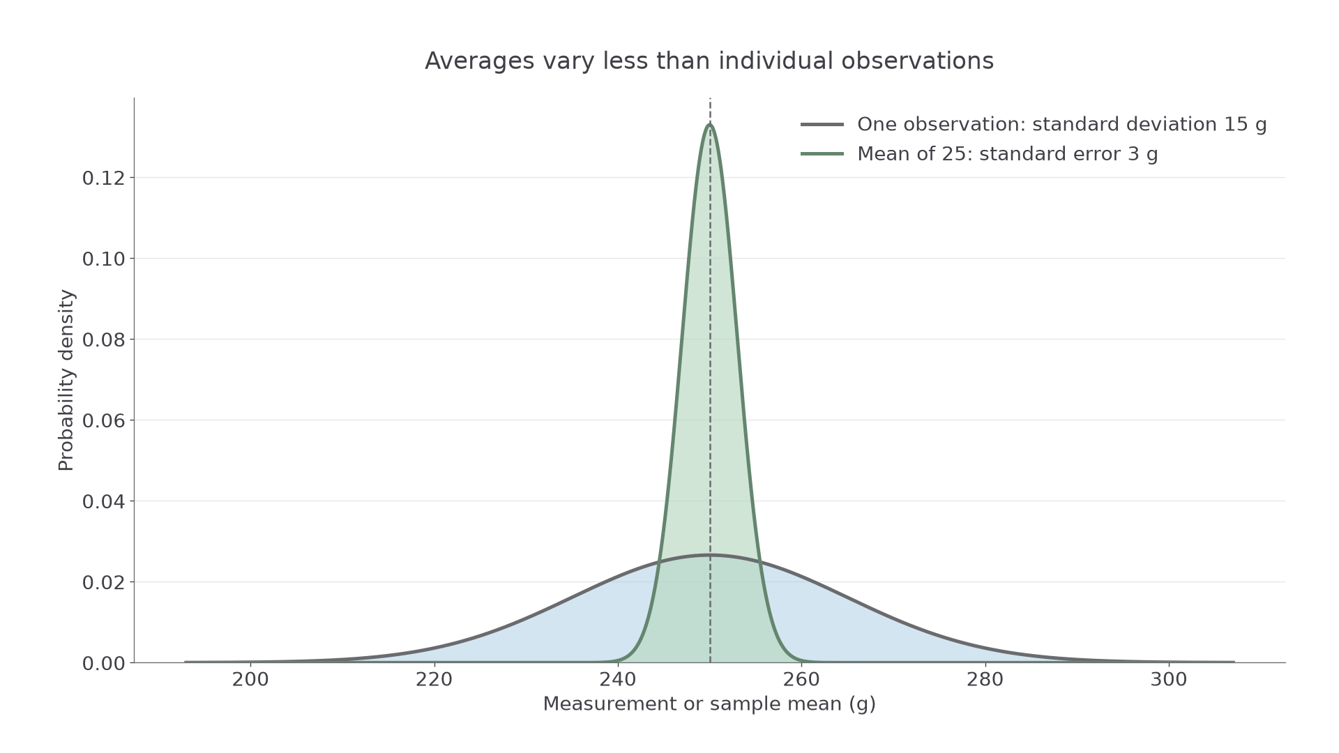
Distributions of individual pack masses and means of twenty-five independent masses

The averages have the same centre, $250$ g, but their standard deviation is $3$ g rather than $15$ g.

Worked example 1: a probability for a mean

Question. Pack masses in grams follow $\mathrm N(250,225)$ . For twenty-five independent packs, find the probability that the sample mean exceeds $256$ g.

Plan. Divide the individual variance by the sample size, then use the resulting standard error.

\begin{aligned} \bar X&\sim\mathrm N(250,225/25)=\mathrm N(250,9)\\ \mathrm P(\bar X>256)&=\mathrm P\!\left(Z>\frac{256-250}{3}\right)\\ &=\mathrm P(Z>2)=0.0227501\ldots \end{aligned}

Why this step? The boundary is two standard errors above the population mean; dividing by the individual standard deviation would answer a different question.

Answer. The probability is about $0.023$ .

Check. The standard error $3$ g is smaller than the individual standard deviation $15$ g, as averaging requires.

Change only the sample size from twenty-five to one hundred, keeping the same population and boundary.

Worked example 2: a tighter sampling distribution

Question. Find the probability that the mean of one hundred independent packs exceeds $256$ g.

Plan. Update the sample-mean variance and standardise again.

\begin{aligned} \bar X&\sim\mathrm N(250,225/100)=\mathrm N(250,2.25)\\ \mathrm P(\bar X>256)&=\mathrm P(Z>4)=0.0000316712\ldots \end{aligned}

Why this step? Quadrupling the sample size halves the standard error to $1.5$ g, doubling the standardised departure.

Answer. The probability is about $0.000032$ .

Check. The same upper departure becomes much less likely for the more tightly concentrated average.

Normality of the population makes this exact; independence still matters. We do not need a theorem about averages from other population shapes to establish this result.

Watch out

Do not put the standard error in the variance position of Normal notation. For twenty-five packs, write $\mathrm N(250,9)$ , not $\mathrm N(250,3)$ .

Try another average with a different measurement scale.

Setting up and carrying out a mean test

A mean test compares the observed average with the distribution it would have if the population mean equalled the null claim.

Define $\mu$ in context. An increase, decrease and any change correspond respectively to $\mathrm H_1:\mu>\mu_0$ , $\mathrm H_1:\mu<\mu_0$ and $\mathrm H_1:\mu\ne\mu_0$ , with $\mathrm H_0:\mu=\mu_0$ . The alternative is chosen before inspecting the sample.

Known-variance mean test

Under $\mathrm H_0:\mu=\mu_0$ , for independent Normal observations with known population standard deviation $\sigma$ ,

\bar X\sim\mathrm N\!\left(\mu_0,\frac{\sigma^2}{n}\right),\qquad z=\frac{\bar x-\mu_0}{\sigma/\sqrt n}.

In the formula sheet.

The lower-tail p-value is $\mathrm P(Z\le z)$ , the upper-tail p-value is $\mathrm P(Z\ge z)$ , and the two-tail normal p-value is $2\mathrm P(Z\ge|z|)$ . These tail choices and the rejection rule are not supplied formulas: learn their meaning. Reject when the p-value is at most the preselected significance level.

Worked example 3: testing for underfilling

Question. Pack masses are Normal with known population standard deviation $15$ g. Twenty-five independently sampled packs have mean $244$ g. Test for a decrease from a claimed population mean of $250$ g at $5\%$ .

Plan. Let $\mu$ be the population mean pack mass in grams. Use the null mean and the standard error of the sample average.

\begin{aligned} \mathrm H_0&:\mu=250,\qquad \mathrm H_1:\mu<250\\ \bar X\mid\mathrm H_0&\sim\mathrm N(250,9)\\ z&=\frac{244-250}{3}=-2\\ \mathrm P(Z\le-2)&=0.0227501\ldots<0.05 \end{aligned}

Why this step? The observed $6$ g decrease is two standard errors, despite being less than one individual standard deviation.

Answer. Reject the null. There is sufficient evidence at $5\%$ to suggest that the population mean pack mass is below $250$ g.

Check. The p-value is a lower tail, matching the planned decrease.

Keep the same test and change only the observed mean to $246$ g.

Worked example 4: a weaker departure

Question. What is the conclusion for an observed mean of $246$ g in the same experiment?

Plan. Use the unchanged standard error and evaluate the new lower tail.

z=\frac{246-250}{3}=-\frac43,\qquad \mathrm P(Z\le-4/3)=0.0912112\ldots>0.05.

Why this step? The null distribution's centre stays at the claimed $250$ , rather than moving to the sample mean.

Answer. Do not reject. There is insufficient evidence at $5\%$ to suggest that the population mean pack mass is below $250$ g.

Check. A smaller observed decrease gives a larger p-value and weaker evidence, consistently with the earlier result.

A normal calculator can work directly with the null sample-mean distribution. Check whether it requests standard deviation or variance, and keep unrounded values until the comparison.

Watch out

Writing the null distribution with centre $\bar x$ makes the observation central by construction. Use $\mu_0$ as its mean; $\bar x$ is the observation being assessed.

Now use an upper tail in a fresh context.

Critical values and two-tailed tests

A critical region describes the sample means that trigger rejection; the acceptance region contains those for which the null is not rejected.

For an upper one-tail test use an upper-tail area $\alpha$ , and for a two-tail test use $\alpha/2$ at each end. A lower one-tail test uses the reflected lower boundary. The supplied table labels the total area in two equal tails: its $5\%$ row gives $1.960$ , not the $5\%$ upper one-tail point $1.645$ .

Sample-mean boundaries

If $c$ is the positive standard normal cutoff matching the required tail area, the sample-mean boundaries are

\mu_0\pm c\frac{\sigma}{\sqrt n}.

Use the relevant one boundary or both outer tails. Standardisation and selected normal percentage points are supplied; this rearranged boundary rule is not printed separately.

Not in the formula sheet: learn it.

The boundaries locate possible averages under a fixed null claim. They are not a confidence interval estimating an unknown population mean.

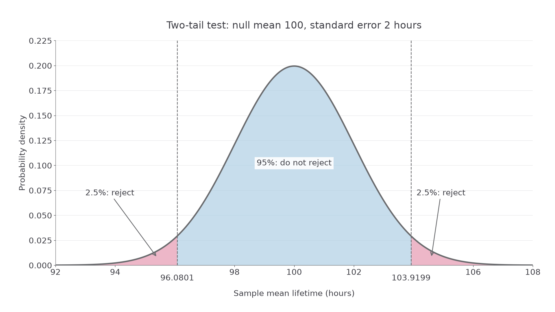
Two outer rejection tails for a normal sample mean centred at one hundred hours

Each tail has probability $0.025$ for the $5\%$ two-tail rule; the central acceptance region has probability $0.95$ .

Worked example 5: a two-tail test at five per cent

Question. Normal lifetimes have known population standard deviation $12$ hours. An independent sample of $36$ has mean $104$ hours. Test $\mathrm H_0:\mu=100$ against $\mathrm H_1:\mu\ne100$ at $5\%$ , using a critical region.

Plan. Use standard error $12/\sqrt{36}=2$ , with $0.025$ in each tail.

100\pm1.95996398\ldots(2)=96.080072\ldots,\ 103.919928\ldots.

Why this step? A change can occur in either direction, so both extreme tails must share the level.

Answer. Reject for $\bar X\le96.080072\ldots$ or $\bar X\ge103.919928\ldots$ ; the acceptance region lies between. Since $104$ lies above the upper boundary, there is sufficient evidence at $5\%$ to suggest that the population mean lifetime differs from $100$ hours.

Check. $z=2$ , giving two-tail p-value $0.0455003\ldots<0.05$ .

Continue this lesson.

You’re previewing NovaLearn without an account. Create a free account to read the rest.

Create free account

Last Accessed

Pure Mathematics

Statistics

Mechanics

MH7–MH9 - The sample mean and normal mean tests

The distribution of a sample mean

Setting up and carrying out a mean test

Critical values and two-tailed tests

Continue this lesson.

Learn faster with Nova