Physics 6.23 - 6.27 - Activity and half-life
A single nucleus decays unpredictably, yet a large source follows a predictable half-life pattern. Use this distinction to interpret activity, read decay graphs and calculate what remains.
Activity and the becquerel
A source contains many unstable, undecayed nuclei. Activity is the rate of nuclear decay in the source. Its unit is the becquerel, :
A source with activity undergoes about 600 decays per second on average; it does not contain only 600 nuclei. Actual numbers in short intervals fluctuate because the decays are random. A GM counter records only the emissions it detects, so its count rate is not automatically equal to the source activity.
As nuclei decay, fewer undecayed nuclei remain. Each surviving nucleus retains the same probability of decaying during the next fixed interval, but there are fewer nuclei available, so fewer decay each second on average. The activity decreases. The surviving nuclei have not become tired or weaker.
The decrease is curved: the same fraction of the current activity is lost in equal intervals, so the absolute decrease becomes smaller as the activity falls. Here we track a single isotope; additional radioactive daughter products would require a more detailed model.
Reading the half-life pattern
The half-life of a radioactive isotope is the time taken for half its undecayed nuclei to decay, or for its activity to fall to half its value. This describes the expected large-sample pattern, not a deadline for each nucleus.
Activity is proportional to the number of undecayed nuclei for the same isotope. Half as many undecayed nuclei means half as many opportunities for decay per second. Every half-life halves the amount currently remaining, not half the original amount again.
| Number of half-lives | Expected fraction remaining |
|---|---|
| 0 | |
| 1 | |
| 2 | |
| 3 | |
| 4 |
[DIAGRAM: asset_slug: physics_6_23_6_27_half_life_activity_and_calculations__diagram_01; description: Expected activity curve starting at 400 Bq, halving every 3 min; points at 3 min and 200 Bq, 6 min and 100 Bq, 9 min and 50 Bq, 12 min and 25 Bq.]
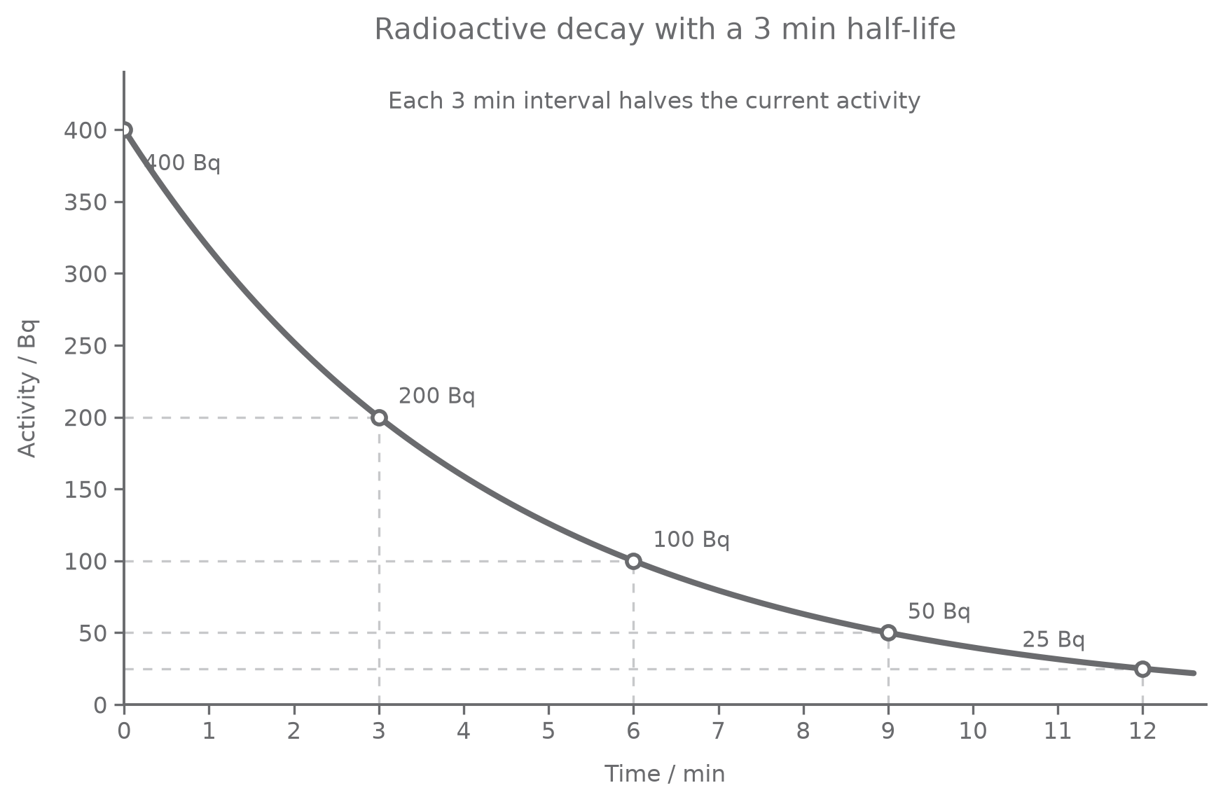
Read a half-life from the graph. Start at , halve it to , move horizontally to the curve and down to read . Check another pair: at falls to at . The interval is , so the half-life is constant.
Half-life is a time difference. Do not simply read the time coordinate unless your chosen interval starts at zero. Read several activity-halving pairs to check an estimate from a noisy graph. Keep the axes and units clear when plotting data, and use a smooth decreasing trend rather than forcing fluctuating measurements onto a straight line. If the graph is a detector count rate, subtract background before halving the source contribution; the measured total approaches background, not zero.
Random nuclei, predictable samples
There is no way to predict exactly when a particular unstable nucleus will decay. Surviving one half-life does not make it overdue: during the next half-life, each surviving nucleus of that isotope still has a probability of of decaying.
Many independent random events create a predictable proportion when the sample is very large. About half remain after one half-life and about a quarter after two; small samples can depart substantially from these expected fractions. Random does not mean that decay has no pattern at the population scale.
The smooth activity curve approaches zero. A finite sample can eventually undergo its last decay, but the time of that last event is random, not fixed by drawing the curve to an axis.
Continue this lesson.
You’re previewing NovaLearn without an account. Create a free account to read the rest.
Create free account