Biology 9.5 - 9.6 - Quadrat and transect fieldwork
Choose representative field samples, investigate an environmental gradient using a belt transect, and turn quadrat counts into population estimates with clear limits.
Samples and quadrats
Counting every organism in a habitat would be a census. That is often too slow and may be impossible, so ecologists count organisms in smaller areas called samples and use those data as evidence about the whole population. A good sample represents the study area: it is large enough, uses the same measurement rule each time and is not placed only where the investigator expects a particular result.
Quadrat
A quadrat is a frame of known area used to define exactly which ground and organisms belong to one sample.
For a low-growing plant whose individuals can be distinguished, place the quadrat flat and count plants rooted inside it. Before collecting data, agree an edge rule, such as counting plants rooted on the top and left edges but not the bottom and right edges. This prevents the same edge plant from being counted twice in neighbouring quadrats.
Where separate individuals cannot be distinguished, such as a spreading moss, a gridded quadrat can estimate percentage cover. Use one agreed rule for every sample. For example, in a grid, 37 squares at least half covered gives an estimated cover of . Percentage cover measures occupied area; it is not the number of organisms.
Random sampling across an area
Random sampling is appropriate when the question asks for abundance across one area, rather than change along a gradient. Mark two perpendicular edges of the study area with tapes to make x and y axes. Generate pairs of random coordinates before looking at the vegetation, place the same corner of the quadrat at each coordinate, count using the agreed rule, and repeat at many different coordinates.
Every valid coordinate must have an equal chance of selection. That reduces selection bias: throwing a quadrat or choosing a patch that "looks typical" can avoid bare ground, awkward edges or dense patches and make the sample unrepresentative.
Choosing a representative sample
Define the target population and boundary first. A preliminary survey helps select a quadrat size that can contain enough identifiable organisms and a sample size that captures patchiness. Include empty quadrats as zero counts. Avoid taking every sample beside an easy path or omitting awkward corners. Choose only coordinates at which the whole quadrat fits within the defined area, using a pre-agreed rule for the boundary.
If a meadow contains a shaded strip covering one quarter of its area and open grass covering three quarters, a purely convenient sample of open grass misses a known habitat. One solution is stratified random sampling: sample randomly within each habitat, in proportion to its area, or calculate a density for each habitat and multiply by its own area before adding the estimates. For example, 8 of 32 quadrats in the shaded strip and 24 in open grass sample the habitats proportionately. More random samples reduce sampling variation; they cannot guarantee an exact census.
Core practical: a belt transect
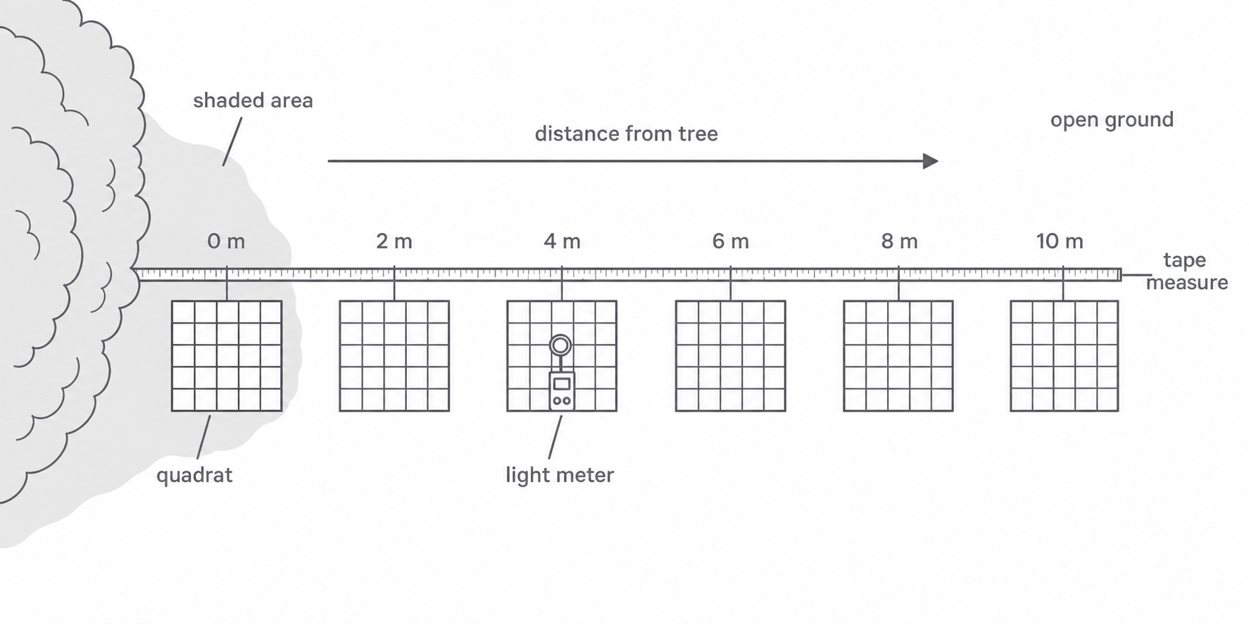
A belt transect answers a different question: how does the distribution or abundance of an organism change along an environmental gradient? A line transect records organisms touching a line. A belt transect samples a strip with quadrats placed next to the line, so it gives quantitative abundance data for a known area.
This investigation asks: what is the relationship between light intensity and the abundance of a named low-growing plant from beneath a tree canopy to open ground? The independent or explanatory variable is light intensity, measured rather than deliberately changed, in lux. Distance along the transect is the systematic sampling position, in metres. The dependent variable is plant abundance, measured as the mean number of target plants per quadrat.
Apparatus and design
Use a 10 m tape measure and pegs, a gridded quadrat, a light meter, a plant identification key and a recording sheet. The quadrat gives the same sampled area each time; the tape locates fixed stations; the light meter turns "shade" into a measured quantity; and the key helps different observers identify the same target species.
[DIAGRAM: asset_name: Biology 9.5-9.6 - Fieldwork sampling with quadrats and transects - diagram 01; asset_slug: biology_9_5_9_6_fieldwork_sampling_with_quadrats_and_transects__diagram_01; recommended_method: image_gen; description: Top-down scientific fieldwork layout on white showing a tree canopy at the shaded left, open ground at the right, one straight tape measure from 0 m to 10 m, equal 2 m stations, identical square quadrats placed on the same side of the tape at each station to form an interrupted belt transect, and a light meter shown at a quadrat centre. Label shaded area, open ground, tape measure, quadrat, light meter and distance from tree; use only white and neutral grey, show one clear left-to-right distance arrow, and include no random quadrat placement, people, decorative data or organisms outside the frames.]
Reproducible method
- Inspect the site before starting. Identify the target plant with a key and agree the rooted-inside and edge-counting rules.
- Lay the tape in a straight line from deep shade beneath the canopy to open ground. A range should include both ends of the light gradient. Keep the tape visible and close to the ground.
- Place one edge of the quadrat against the tape at , always on the same side. Count the target plants without uprooting them.
- Put the light-meter sensor at the centre of the quadrat, at the same height and orientation each time. Keep your body from shading the sensor. Allow the reading to settle, then record light intensity in lux beside the plant count and distance. Make identification notes or photographs for uncertain specimens rather than guessing; resolve them using the key.
- Repeat the plant count and light reading at intervals up to . These fixed positions make this an interrupted belt transect, not a random sample.
- Repeat the whole procedure with at least two more parallel transects through the same type of shaded-to-open habitat. Keep transect length, interval, quadrat area, target species, edge rule and measuring technique the same.
- Record every result, including an unexpected one. Recheck a surprising light reading or identification and note an observable cause; do not remove a value merely because it does not fit the pattern.
The interval balances detail against fieldwork time. A smaller interval would give more spatial detail but take longer; a wider interval could miss a narrow change. The repeat transects sample natural patchiness, rather than measuring the same small strip repeatedly.
Safety and care for the habitat
Uneven ground and the long tape create trip risks: check the route, wear closed footwear, keep the tape visible and walk beside it rather than over it. Cover skin where prickly or stinging plants may be present, do not touch unidentified organisms, and wash hands after fieldwork. Count plants in place, lift and replace the quadrat carefully, and minimise trampling so that measuring the population does not damage it.
From readings to a conclusion
Raw data should keep paired measurements together: distance, light intensity and plant count from the same quadrat belong in the same row. Repeats should remain visible before a mean is calculated, so variation and possible anomalies are not hidden. In the processed summary below, the three counts come from three parallel transects and each light value is the mean of the three corresponding light readings; the original paired readings must still be kept in the field table.
| Distance from canopy / m | Mean light intensity / lux | Count 1 | Count 2 | Count 3 | Mean count per quadrat |
|---|---|---|---|---|---|
| 0 | 120 | 1 | 2 | 1 | 1.3 |
| 2 | 260 | 2 | 3 | 2 | 2.3 |
| 4 | 480 | 4 | 5 | 4 | 4.3 |
| 6 | 690 | 7 | 6 | 8 | 7.0 |
| 8 | 860 | 9 | 10 | 8 | 9.0 |
| 10 | 940 | 10 | 11 | 9 | 10.0 |
Worked example: calculate a mean
At , the three counts are 7, 6 and 8 plants. A mean represents the average count for that station:
Arithmetic mean
The unit is plants per quadrat, not plants per square metre, because area has not yet been used to calculate density. The result is sensible because 7.0 lies within the three observed counts, from 6 to 8.
Raw transect counts can also determine the number actually observed in the sampled belt. Suppose five non-overlapping quadrats contain 1, 2, 4, 7 and 9 plants. The sampled area is , and the number recorded in that area is . Keep the separate position counts as well as the total, because their order shows how distribution changes along the gradient.
To test the measured relationship, plot light intensity in lux on the x-axis and mean plant count per quadrat on the y-axis. Use a scatter graph because each point is a pair of measured variables; do not join points dot-to-dot. A line of best fit can show the overall trend.
The table shows a positive correlation: higher light intensity is associated with a higher mean count of this plant. That is an observation supported by the paired data. It does not by itself prove that light caused the change because soil moisture, soil pH, trampling or another factor might also vary along the transect. A conclusion should therefore describe the relationship and its limits, rather than claiming that all plant species prefer high light.
Continue this lesson.
You’re previewing NovaLearn without an account. Create a free account to read the rest.
Create free account