Physics 2.6 - 2.7, 2.11 - 2.12 - Speed and its measurement

Speed, distance and time

Imagine timing a runner from the start line to the finish. The distance travelled is the total length of the route, measured in metres ($\mathrm{m}$). The elapsed time is the duration of the journey, measured in seconds ($\mathrm{s}$). Average speed tells us how much distance was travelled per second across the whole measured interval.

The unit follows from the division: $\mathrm{m}/\mathrm{s}=\mathrm{m\,s^{-1}}$. A speed of $5\,\mathrm{m\,s^{-1}}$ means that the object covers an average of 5 metres in each second of that interval. It does not mean the speed was exactly $5\,\mathrm{m\,s^{-1}}$ at every instant.

Worked example: calculating average speed

A runner travels $750\,\mathrm{m}$ in $150\,\mathrm{s}$.

1. The quantities already use metres and seconds, so no conversion is needed.
2. Select $\text{average speed}=\frac{\text{distance}}{\text{time}}$.
3. Substitute: $v = 750 / 150$.
4. Calculate: $v = 5.0\,\mathrm{m\,s^{-1}}$.
5. Sense-check: at $5.0\,\mathrm{m\,s^{-1}}$, 150 seconds would give $5.0 \times 150 = 750\,\mathrm{m}$, so the value is consistent.

The same relationship can be rearranged to find distance:

Worked example: calculating distance

A travelator carries a passenger at an average speed of $1.2\,\mathrm{m\,s^{-1}}$ for $45\,\mathrm{s}$.

1. Select $d = vt$.
2. Substitute: $d = 1.2 \times 45$.
3. Calculate: $d = 54\,\mathrm{m}$.
4. Sense-check: just over 1 metre each second for 45 seconds should be just over 45 metres, so 54 metres is plausible.

Do not calculate average speed by simply adding a starting speed and a finishing speed and dividing by two. That shortcut works only in particular kinds of motion. The definition that always applies here is total distance divided by total time.

Distance-time graphs

A distance-time graph records the distance already travelled at each time. Time is on the horizontal axis and distance is on the vertical axis. Before interpreting a line, read both axis quantities and units: the graph is a mathematical record of motion, not a side-view picture of a road or hill.

• A rising straight line means distance increases by an equal amount in each equal time interval: constant speed.
• A steeper line means more distance is covered per second: greater speed.
• A horizontal line means distance is not changing: the object is stationary.
• A curved line means the gradient, and therefore the speed, is changing.

Because distance travelled accumulates, it does not decrease. A downward line would not be a valid distance-travelled graph.

[DIAGRAM: asset_name: Physics 2.6-2.13 - Speed, acceleration and motion graphs - diagram 01; asset_slug: physics_2_6_2_13_speed_acceleration_and_motion_graphs__diagram_01; recommended_method: matplotlib; description: Exact distance-time graph on a white background with #6A6B6E axes and line, showing points ($0\,\mathrm{s}$, $0\,\mathrm{m}$), ($4\,\mathrm{s}$, $12\,\mathrm{m}$), ($6\,\mathrm{s}$, $12\,\mathrm{m}$) and ($10\,\mathrm{s}$, $20\,\mathrm{m}$); label the three straight sections 'constant speed: $3\,\mathrm{m\,s^{-1}}$', 'stationary' and 'constant speed: $2\,\mathrm{m\,s^{-1}}$'; time horizontal in s, distance vertical in m; no downward segment, decorative marks or colour-dependent meaning.]

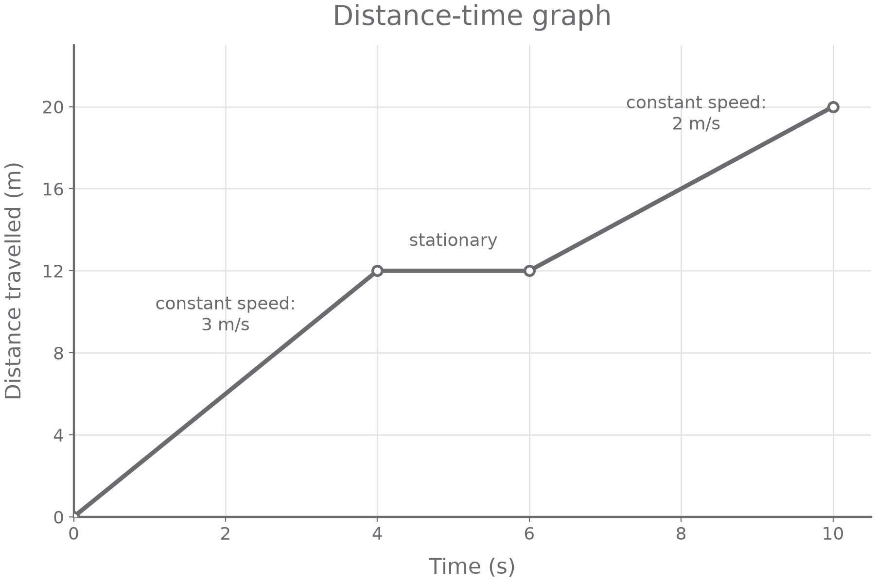
Worked example: reading the journey

For the first section of the graph, choose the endpoints $(0\,\mathrm{s}, 0\,\mathrm{m})$ and $(4\,\mathrm{s}, 12\,\mathrm{m})$:

$\text{speed}=\frac{12-0}{4-0}=\frac{12}{4}=3\,\mathrm{m\,s^{-1}}$

From $4\,\mathrm{s}$ to $6\,\mathrm{s}$, distance remains $12\,\mathrm{m}$, so $\text{change in distance}=0\,\mathrm{m}$ and the speed is $0\,\mathrm{m\,s^{-1}}$.

For the final section, use $(6\,\mathrm{s}, 12\,\mathrm{m})$ and $(10\,\mathrm{s}, 20\,\mathrm{m})$:

$\text{speed}=\frac{20-12}{10-6}=\frac{8}{4}=2\,\mathrm{m\,s^{-1}}$

The first rising section is steeper than the last, matching the numerical comparison $3\,\mathrm{m\,s^{-1}} > 2\,\mathrm{m\,s^{-1}}$. Notice that using $20 / 10$ would give an average for the whole journey, including the stop; it would not give the speed on the final section.