3.02e, 3.02g, 1.10h - Motion in two dimensions with vectors | OCR A-Level Mathematics A

Track a particle in a plane using two components that share one clock. Use constant-acceleration equations or calculus to find position and velocity, then distinguish the route travelled from the displacement between its endpoints.

Position, travel and direction in a plane

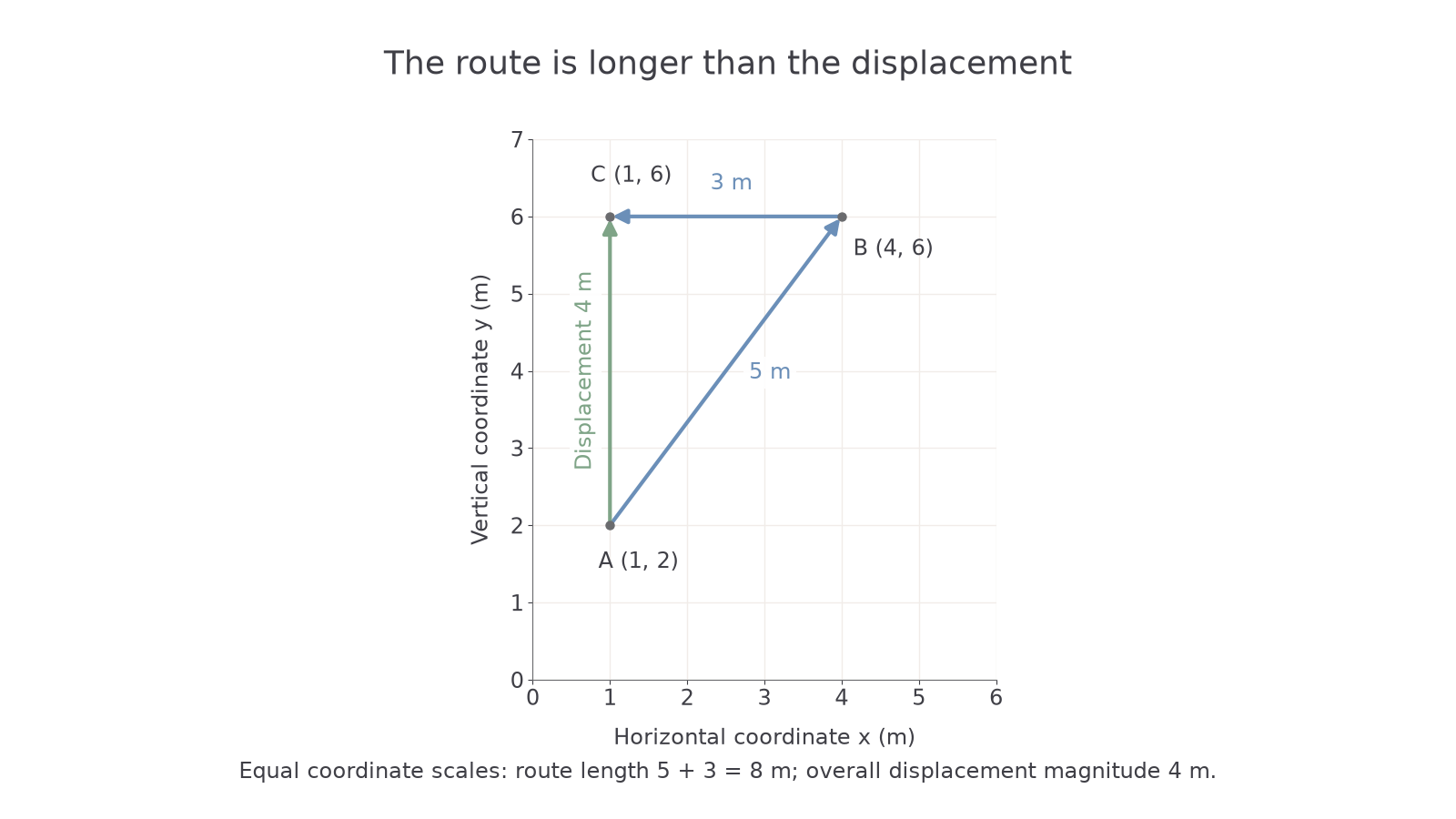
Can a particle travel eight metres in four seconds while its average velocity has magnitude only one metre per second? Start at $A=(1,2)$ , travel straight to $B=(4,6)$ , then straight to $C=(1,6)$ , with coordinates in metres. The route takes a detour; the displacement cuts straight from start to finish.

You already know

Subtract position vectors in destination-minus-start order. For perpendicular components, $|p\mathbf i+q\mathbf j|=\sqrt{p^2+q^2}$ . A vector has direction as well as magnitude.

Here $\mathbf i$ and $\mathbf j$ are fixed perpendicular unit vectors along positive horizontal coordinate axes. A position such as $\mathbf x=\mathbf i+2\mathbf j$ can also be written $\begin{pmatrix}1\\2\end{pmatrix}$ . Units belong to the physical vector, not to the unit vectors themselves.

[DIAGRAM: asset_name: A route and its overall displacement; asset_slug: vector_route; description: Equal-scale coordinate diagram showing A(1,2), B(4,6), C(1,6), the 5 and 3 metre legs and the 4 metre displacement from A to C; caption: A route and its overall displacement]

Position, displacement and distance

Position locates a particle relative to a fixed origin. Displacement is final position minus initial position. Distance from the origin is the magnitude of position; distance travelled is the length of the actual route. A closed trip has zero displacement even when its distance travelled is positive.

Velocity is the rate of change of position; speed is its non-negative magnitude. Acceleration is the rate of change of velocity, including any change of direction. Thus $\mathbf v=-3\mathbf i+4\mathbf j$ has speed $5$ , while its direction is $53.1^\circ$ above the negative horizontal axis. Position need not point in that direction. In a plane, the signs of individual velocity and acceleration components alone do not determine whether speed increases or decreases: consider the combined motion, rather than importing a one-dimensional sign rule.

Averages over a journey

For an elapsed time $T>0$ ,

\text{average velocity}=\frac{\text{overall displacement}}{T},\qquad \text{average speed}=\frac{\text{distance travelled}}{T}

The magnitude of average velocity need not equal average speed. Not in the formula sheet: learn it.

Use a separate length calculation for each straight leg, then add those lengths.

Worked example 1: the eight-metre detour

Question. The journey $A=(1,2)$ to $B=(4,6)$ to $C=(1,6)$ takes $4\,\mathrm s$ . Find the displacement, distance travelled, average velocity and average speed.

Plan. Subtract the endpoints for displacement and add the two leg lengths for distance.

\begin{aligned} \overrightarrow{AC}&=(1-1)\mathbf i+(6-2)\mathbf j=4\mathbf j && \text{end minus start}\\ AB&=\sqrt{3^2+4^2}=5 && \text{first leg}\\ BC&=3 && \text{horizontal return}\\ \text{distance travelled}&=5+3=8 && \text{add leg lengths}\\ \text{average velocity}&=4\mathbf j/4=\mathbf j && \text{displacement per second}\\ \text{average speed}&=8/4=2 && \text{distance per second} \end{aligned}

Why this step? Displacement ignores the detour, but distance records it.

Answer. Displacement is $4\mathbf j\,\mathrm m$ ; distance travelled is $8\,\mathrm m$ . Average velocity is $\mathbf j\,\mathrm{m\,s^{-1}}$ , and average speed is $2\,\mathrm{m\,s^{-1}}$ .

Check. The endpoint separation is $4\,\mathrm m$ , less than the route length $8\,\mathrm m$ . The final distance from the origin is instead $\sqrt{37}\,\mathrm m$ .

Change only the final point to the starting point. The same requests now reveal a striking boundary case: a moving particle can have zero average velocity.

Worked example 2: a closed journey

Question. The journey $A=(1,2)$ to $B=(4,6)$ to $A=(1,2)$ takes $4\,\mathrm s$ . Find the displacement, distance travelled, average velocity and average speed.

Plan. Keep displacement and distance separate, even though the endpoints coincide.

\begin{aligned} \text{displacement}&=(1-1)\mathbf i+(2-2)\mathbf j=\mathbf0 && \text{same endpoints}\\ \text{distance travelled}&=5+5=10 && \text{out and back}\\ \text{average velocity}&=\mathbf0/4=\mathbf0 && \text{divide displacement}\\ \text{average speed}&=10/4=2.5 && \text{divide distance} \end{aligned}

Why this step? Zero displacement says where the journey ends, not whether the particle moved.

Answer. Displacement and average velocity are zero vectors; distance travelled is $10\,\mathrm m$ , and average speed is $2.5\,\mathrm{m\,s^{-1}}$ .

Check. The two displacement vectors cancel, while both leg lengths are positive.

A curved or turning route can make these quantities differ just as sharply.

Watch out

Wrong: average speed is $|\overrightarrow{AC}|/T$ for every route. That is the magnitude of average velocity. Add the route lengths before dividing to find average speed.

Try a new out-and-back route; the elapsed time is unchanged.

Constant acceleration with vector equations

A constant acceleration vector lets each component use its one-dimensional equations over the same elapsed time.

You already know

The scalar constant-acceleration equations require acceleration to stay constant throughout the interval. Displacement measures change of position, so add the starting position afterwards.

If $\mathbf a=a_x\mathbf i+a_y\mathbf j$ is constant, integrating its components gives $v_x=u_x+a_xt$ and $v_y=u_y+a_yt$ . Combining those results gives the first vector equation below; integrating once more gives the displacement equation. The other two follow by substitution.

Constant acceleration in a plane

For constant $\mathbf a$ ,

\begin{aligned} \mathbf v&=\mathbf u+\mathbf a t\\ \mathbf s&=\mathbf u t+\tfrac12\mathbf a t^2\\ \mathbf s&=\tfrac12(\mathbf u+\mathbf v)t\\ \mathbf s&=\mathbf v t-\tfrac12\mathbf a t^2 \end{aligned}

Here $\mathbf s=\mathbf x(t)-\mathbf x(0)$ . In the formula sheet.

There is no componentwise vector-square equation to add to this list. The dot-product extension of the squared-speed equation is excluded here; work with these vector equations or a scalar equation along one chosen axis.

Worked example 3: displacement before position

Question. A particle starts at $\mathbf i+4\mathbf j\,\mathrm m$ , with velocity $3\mathbf i-2\mathbf j\,\mathrm{m\,s^{-1}}$ and constant acceleration $-\mathbf i+2\mathbf j\,\mathrm{m\,s^{-2}}$ . Find its velocity and position after $2\,\mathrm s$ .

Plan. Use the common time in both vector equations, then add the initial position.

\begin{aligned} \mathbf v&=\begin{pmatrix}3\\-2\end{pmatrix}+2\begin{pmatrix}-1\\2\end{pmatrix}=\begin{pmatrix}1\\2\end{pmatrix} && \text{velocity change}\\ \mathbf s&=2\begin{pmatrix}3\\-2\end{pmatrix}+\tfrac12(2^2)\begin{pmatrix}-1\\2\end{pmatrix}=\begin{pmatrix}4\\0\end{pmatrix} && \text{displacement}\\ \mathbf x(2)&=\begin{pmatrix}1\\4\end{pmatrix}+\begin{pmatrix}4\\0\end{pmatrix}=\begin{pmatrix}5\\4\end{pmatrix} && \text{add starting position} \end{aligned}

Why this step? The displacement formula measures from the starting point, which is not the origin.

Answer. Velocity is $\mathbf i+2\mathbf j\,\mathrm{m\,s^{-1}}$ ; position is $5\mathbf i+4\mathbf j\,\mathrm m$ .

Check. The average-velocity formula gives $\tfrac12[(3,-2)+(1,2)](2)=(4,0)$ , the same displacement.

Change only the initial position. Velocity and displacement should stay exactly the same.

Worked example 4: shifting the starting point

Question. A particle starts at $-2\mathbf i+\mathbf j\,\mathrm m$ , with velocity $3\mathbf i-2\mathbf j\,\mathrm{m\,s^{-1}}$ and constant acceleration $-\mathbf i+2\mathbf j\,\mathrm{m\,s^{-2}}$ . Find its velocity and position after $2\,\mathrm s$ .

Plan. Reuse the velocity and displacement calculation, then translate by the new starting position.

\begin{aligned} \mathbf v&=(3-2)\mathbf i+(-2+4)\mathbf j=\mathbf i+2\mathbf j && \text{same initial velocity}\\ \mathbf s&=(6-2)\mathbf i+(-4+4)\mathbf j=4\mathbf i && \text{same acceleration and time}\\ \mathbf x(2)&=(-2\mathbf i+\mathbf j)+4\mathbf i=2\mathbf i+\mathbf j && \text{new initial position} \end{aligned}

Why this step? Translating the entire motion changes where the particle is, without changing how it moves.

Answer. Velocity is $\mathbf i+2\mathbf j\,\mathrm{m\,s^{-1}}$ ; position is $2\mathbf i+\mathbf j\,\mathrm m$ .

Check. Both the starting and final positions have shifted by $-3\mathbf i-3\mathbf j\,\mathrm m$ from example 3.

An unknown constant acceleration can instead be recovered from $\mathbf a=(\mathbf v-\mathbf u)/t$ , for $t>0$ . For instance, $(2,1)$ changing to $(8,-2)$ over three seconds gives $\mathbf a=(2,-1)\,\mathrm{m\,s^{-2}}$ ; this is a rearrangement of the supplied equation.

Watch out

Wrong: $\mathbf x=\mathbf u t+\tfrac12\mathbf a t^2$ regardless of starting point. Right: $\mathbf x=\mathbf x(0)+\mathbf u t+\tfrac12\mathbf a t^2$ .

Keep the motion data fixed again and change the starting point yourself.

Differentiate vector components

Differentiate each position component while the fixed unit vectors remain unchanged.

You already know

Differentiate powers of time using the power rule. A constant position component has derivative zero; the speed is the magnitude of velocity.

Apply that familiar scalar rule separately to the two coordinates.

Position, velocity and acceleration

For $\mathbf x=f(t)\mathbf i+g(t)\mathbf j$ ,

\begin{aligned} \mathbf v&=\frac{\mathrm d\mathbf x}{\mathrm dt}=f'(t)\mathbf i+g'(t)\mathbf j\\ \mathbf a&=\frac{\mathrm d\mathbf v}{\mathrm dt}=f''(t)\mathbf i+g''(t)\mathbf j\\ \text{speed}&=|\mathbf v|=\sqrt{f'(t)^2+g'(t)^2} \end{aligned}

Dots such as $\dot{\mathbf x}$ also denote time derivatives. Not in the formula sheet: learn it.

Take the magnitude after differentiation. Differentiating $|\mathbf x|$ gives the rate of change of distance from the origin, which generally differs from speed along the route. A particle moving around a circle centred on the origin makes that distinction vivid: its distance from the origin is constant while it keeps moving.

Continue this lesson.

You’re previewing NovaLearn without an account. Create a free account to read the rest.

Create free account

Last Accessed

Pure Mathematics

Statistics

Mechanics

3.02e, 3.02g, 1.10h - Motion in two dimensions with vectors

Position, travel and direction in a plane

Constant acceleration with vector equations

Differentiate vector components

Continue this lesson.

Learn faster with Nova