1.02d, 1.02e - Quadratic graphs and the discriminant | OCR A-Level Mathematics A

Use 1.02e's completing-the-square method to uncover a quadratic's turning point and symmetry. Then connect those features to 1.02d's graphs and discriminant, so you can classify real roots and determine conditions on an unknown coefficient.

Completing the square

Can $2x^2-12x+11$ ever be as small as $-8$ , for real $x$ ? At $x=0$ it is $11$ , and at $x=3$ it is $-7$ . Trying values suggests a minimum, but completing the square will prove where the expression stops decreasing.

You already know

$(x+p)^2=x^2+2px+p^2$ , and a real square is non-negative. Expanding an expression checks an identity for every real input; checking one input alone cannot do that.

We want to expose a square without changing the expression's value. The linear term tells us which number belongs inside the bracket.

Quadratic function

A quadratic function has the form $\mathrm f(x)=ax^2+bx+c$ , where $a,b,c$ are real constants and $a\ne0$ . Its graph is a parabola. If $a=0$ , the expression is not quadratic.

For a leading coefficient of one, halve the coefficient of $x$ , put that number in the bracket, then compensate for the constant its square introduces.

Worked example 1: a leading coefficient of one

Question. Complete the square in $x^2+6x+2$ .

Plan. Use $(x+3)^2$ , then remove the extra $9$ .

\begin{aligned} x^2+6x+2 &=(x+3)^2-9+2 && \text{half of }6\text{ is }3\\ &=(x+3)^2-7 && \text{collect constants} \end{aligned}

Why this step? $(x+3)^2$ introduces $9$ , which must be subtracted to keep an identity.

Answer. $(x+3)^2-7$ .

Check. Expanding gives $x^2+6x+9-7=x^2+6x+2$ .

Change only the leading coefficient from one to two. First factor it out of the two variable terms; the bracket's linear coefficient changes as a result.

Worked example 2: a leading coefficient of two

Question. Complete the square in $2x^2+6x+2$ .

Plan. Factor out $2$ from the variable terms, then complete the square inside the bracket.

\begin{aligned} 2x^2+6x+2 &=2(x^2+3x)+2 && \text{factor variable terms}\\ &=2\left((x+\tfrac32)^2-\tfrac94\right)+2 && \text{complete inside}\\ &=2(x+\tfrac32)^2-\tfrac52 && \text{multiply the correction} \end{aligned}

Why this step? The correction $-9/4$ is inside a bracket multiplied by two, so it contributes $-9/2$ .

Answer. $2(x+\tfrac32)^2-\tfrac52$ .

Check. Expanding gives $2x^2+6x+9/2-5/2=2x^2+6x+2$ .

The same reasoning works for any nonzero leading coefficient and gives a useful general identity.

Completed-square form

For real $a,b,c$ , with $a\ne0$ ,

ax^2+bx+c =a\left(x+\frac{b}{2a}\right)^2+c-\frac{b^2}{4a}.

This has the form $a(x+p)^2+q$ .

Not in the formula sheet: learn it.

Even integer coefficients can hide a fractional turning point: $x^2+x=(x+\tfrac12)^2-\tfrac14$ . Its least real value is $-1/4$ , although its values at the neighbouring integers $-1$ and $0$ are both zero.

Watch out

Wrong: $2((x-3)^2-9)+11=2(x-3)^2+2$ . Right: $2((x-3)^2-9)+11=2(x-3)^2-7$ . The outside coefficient multiplies the correction too.

Try changing the leading coefficient once more. Leave the linear and constant terms as they were.

Turning points and sketches

Completed-square form turns the algebra into a picture: the square identifies the symmetry line and the greatest or least height.

At $x=-p$ , the bracket $x+p$ is zero. Moving equal distances left or right gives the same square, so the graph is symmetric about that vertical line.

Turning point and line of symmetry

The turning point, or vertex, of $y=a(x+p)^2+q$ is $(-p,q)$ , and its line of symmetry is $x=-p$ . It is a minimum if $a>0$ and a maximum if $a<0$ . For example, $y=2(x+3)^2-7$ has a minimum at $(-3,-7)$ , not $(3,-7)$ .

The vertex height follows because a real square is non-negative. For unrestricted real $x$ , the outputs satisfy $y\ge q$ when $a>0$ , or $y\le q$ when $a<0$ . These vertex, symmetry and bound results are not in the formula sheet: learn them.

Worked example 3: three forms of one curve

Question. Find the turning point, symmetry line and axis intercepts of $y=-x^2+4x+5$ , and describe its shape.

Plan. Complete the square for the turning point, and factorise for the horizontal intercepts.

\begin{aligned} y&=-(x-2)^2+9 && \text{complete the square}\\ y&=-(x-5)(x+1) && \text{factorise}\\ y(0)&=5 && \text{vertical intercept} \end{aligned}

Why this step? Each form exposes a different feature of exactly the same curve.

Answer. The maximum is $(2,9)$ , the symmetry line is $x=2$ , and the intercepts are $(-1,0),(5,0),(0,5)$ . The parabola opens downwards.

Check. The roots are each $3$ units from $x=2$ ; substitution gives $y(2)=9$ .

A downward parabola with its intercepts, maximum and symmetry line labelled

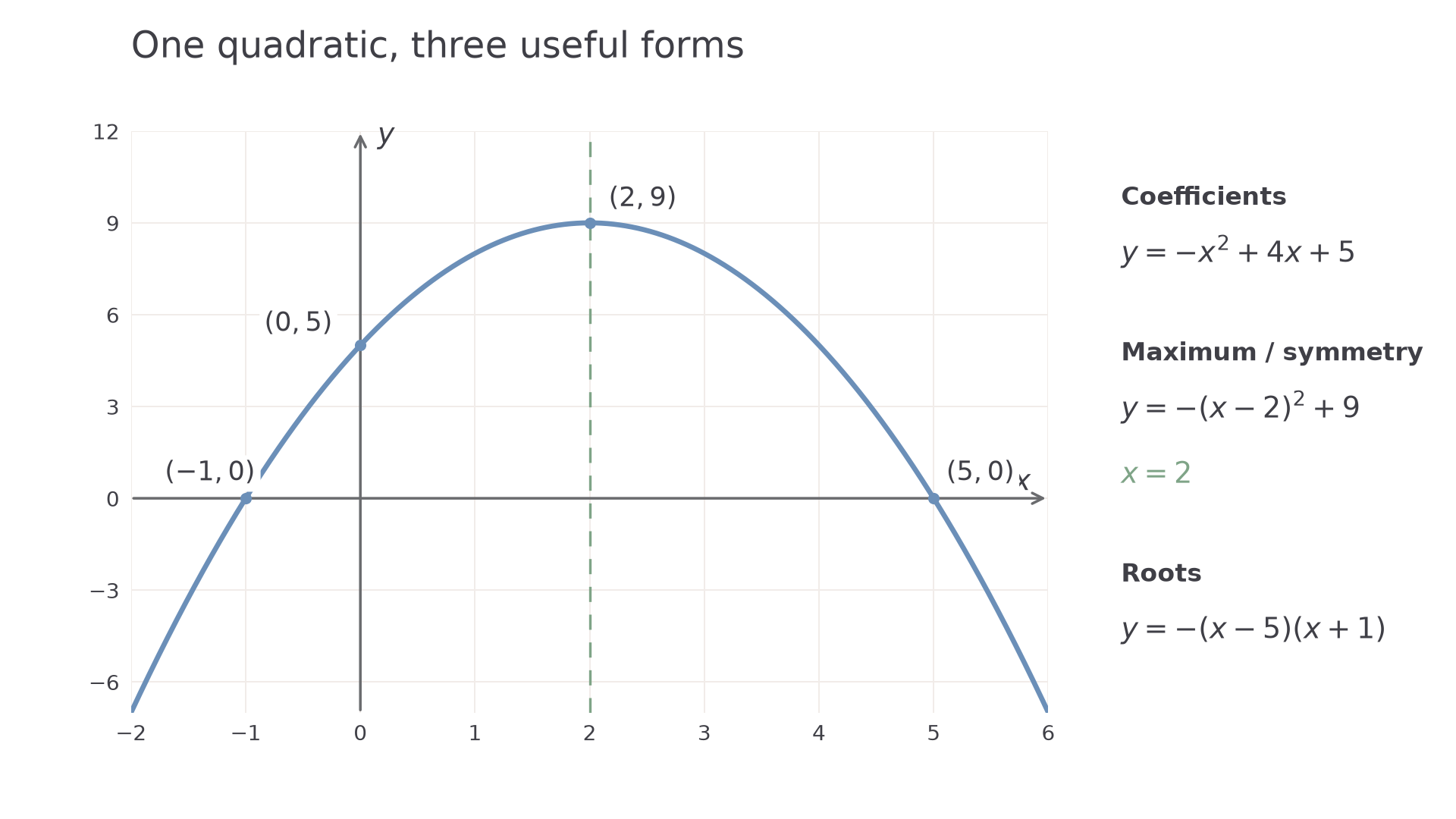
One graph, three forms: coefficients, turning point and roots each become clear in the appropriate form.

Change only the overall sign of the function for the next example. This reflects every height in the horizontal axis, leaving the roots in place.

Worked example 4: reversing the overall sign

Question. Find the turning point, symmetry line and axis intercepts of $y=x^2-4x-5$ , and describe its shape.

Plan. Negate the preceding forms, then read the features.

\begin{aligned} y&=(x-2)^2-9 && \text{complete the square}\\ y&=(x-5)(x+1) && \text{factorise}\\ y(0)&=-5 && \text{vertical intercept} \end{aligned}

Why this step? Negating the function changes $y$ to $-y$ , so the maximum becomes a minimum while zero heights remain zero.

Answer. The minimum is $(2,-9)$ , the symmetry line is $x=2$ , and the intercepts are $(-1,0),(5,0),(0,-5)$ . The parabola opens upwards.

Check. Substituting $x=2$ gives $4-8-5=-9$ ; both factors confirm the same two roots.

A sketch uses labelled axes, intercepts and vertex in the correct relative positions, joined with a smooth parabola. Continue both branches: a quadratic is neither a V nor a semicircle. Equal axis scales are unnecessary for a sketch, but the labelled coordinates must agree with the algebra.

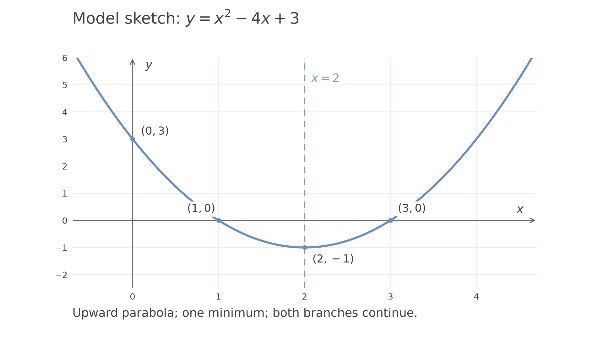
A model upward quadratic sketch with its roots, intercept and minimum labelled

For $y=x^2-4x+3=(x-2)^2-1$ , the roots $1$ and $3$ surround the minimum symmetrically.

Graphing software offers a useful check if the window includes the vertex and intercepts. A narrow window can hide a root; a cursor reading is not an exact derivation.

Watch out

Wrong: the vertex of $y=(x+3)^2-9$ is $(3,-9)$ . Right: it is $(-3,-9)$ , because $x+3=0$ at $x=-3$ . Find where the bracket vanishes rather than copying its sign.

Move the bracket's zero in the last worked example, keeping the height and opening unchanged.

The discriminant and real roots

The discriminant tells you how often a quadratic meets the horizontal axis, without first calculating its roots.

A root of $ax^2+bx+c=0$ is the horizontal coordinate of an axis intersection. A curve can cross twice, touch once, or miss the axis entirely.

Discriminant

For a quadratic with coefficients $a,b,c$ and $a\ne0$ , its discriminant is $\Delta=b^2-4ac$ ; $D$ is another common symbol. Include each coefficient's sign when substituting.

Completing the square explains why its sign matters. Setting the general completed-square form equal to zero gives

\left(x+\frac{b}{2a}\right)^2=\frac{b^2-4ac}{4a^2}.

The denominator on the right is positive. A real square can equal a positive number in two ways, zero in one way, and a negative number in no way.

Discriminant and real roots

For $ax^2+bx+c=0$ , with $a\ne0$ ,

\begin{array}{c|l} \Delta>0&\text{two distinct real roots}\\ \Delta=0&\text{one repeated real root}\\ \Delta<0&\text{no real roots} \end{array}

A repeated root counts twice algebraically but gives only one distinct intercept.

Not in the formula sheet: learn it.

The sign gives the classification; a factorisation or completed square can then check it independently.

Worked example 5: no real roots

Question. Use the discriminant to determine the number of real roots of $x^2-4x+7=0$ .

Plan. Substitute the signed coefficients and interpret the result.

\begin{aligned} \Delta&=(-4)^2-4(1)(7) && \text{identify }a,b,c\\ &=16-28=-12 && \text{evaluate} \end{aligned}

Why this step? A negative discriminant would require a real square to be negative, so no real input can give zero.

Answer. There are no real roots; the graph misses the horizontal axis.

Check. $x^2-4x+7=(x-2)^2+3>0$ , so it is always above the axis.

Change only the constant from $7$ to $4$ . Watch the minimum reach the axis.

Worked example 6: the boundary case

Question. Use the discriminant to determine the number of real roots of $x^2-4x+4=0$ .

Plan. Recalculate the discriminant, then check the factorisation.

\begin{aligned} \Delta&=(-4)^2-4(1)(4) && \text{substitute}\\ &=16-16=0 && \text{evaluate}\\ x^2-4x+4&=(x-2)^2 && \text{check the repeated factor} \end{aligned}

Why this step? Zero on the right of the squared equation gives only one distinct real value, counted as a repeated root.

Answer. The repeated real root is $x=2$ ; the graph touches the axis at its minimum.

Check. Substituting $2$ gives $4-8+4=0$ .

For comparison, $2x^2+x-3=(2x+3)(x-1)$ has $\Delta=25>0$ , consistent with roots $-3/2$ and $1$ . Also, $9x^2-12x+4=(3x-2)^2$ has $\Delta=0$ , with repeated root $2/3$ .

Three parabolas linking the sign of the discriminant to crossings, touching and no intercept

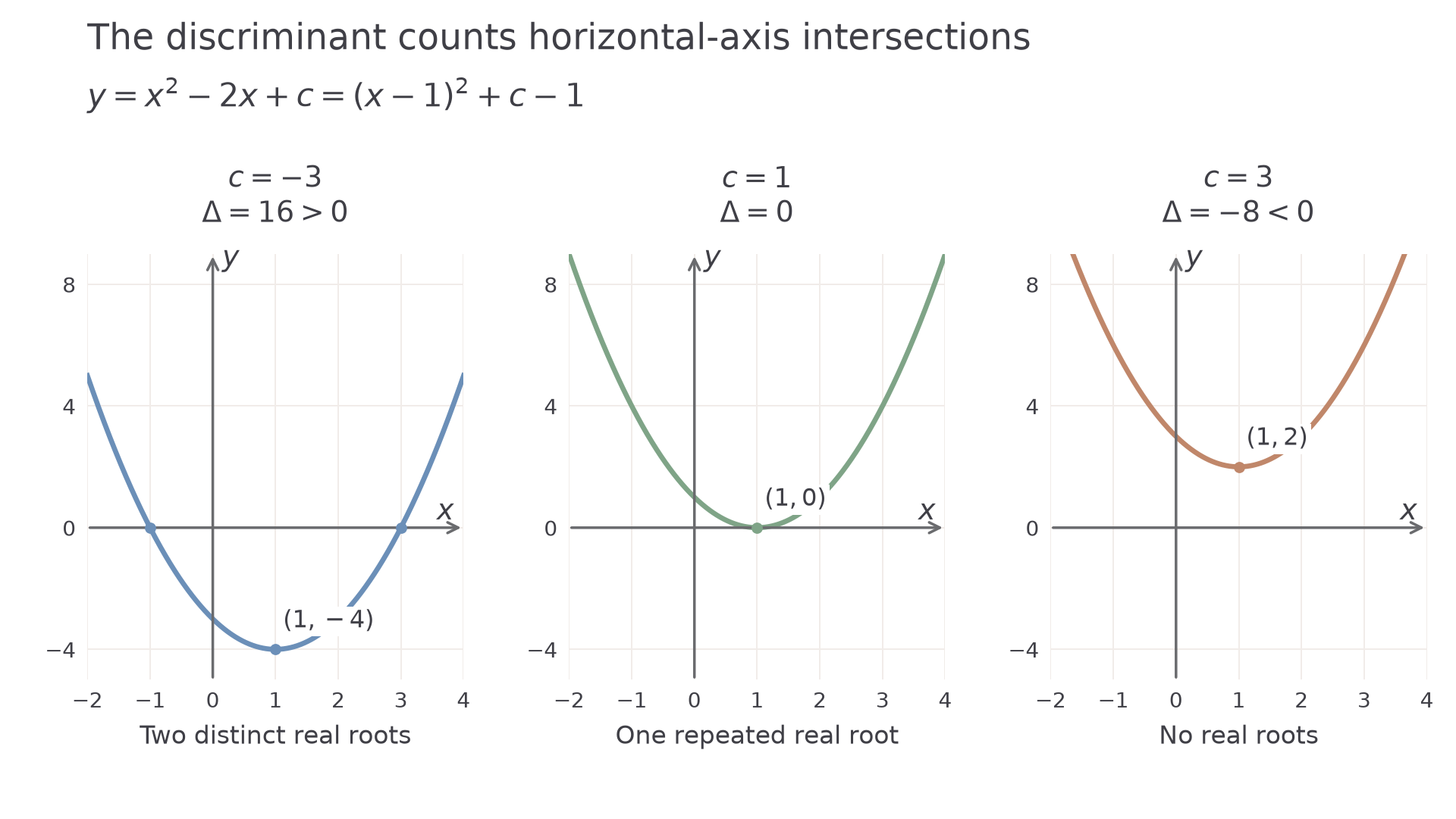
For $y=x^2-2x+c$ , changing $c$ moves the minimum through the horizontal axis.

A negative discriminant does not tell you which side of the axis the graph occupies. If $a>0$ , its minimum is positive; if $a<0$ , its maximum is negative.

Watch out

Wrong: $\Delta<0$ means “there is no graph”. Right: the quadratic has a real graph but no real roots. Do not seek non-real roots here; the conclusion about real intersections is complete.

Change the constant once more and include the graph interpretation with your classification.

Conditions on a coefficient

A condition about roots becomes a condition on the discriminant, so you can classify a whole family of quadratics at once.

For $y=x^2-2x+c=(x-1)^2+c-1$ , the minimum is below, on or above the axis as $c<1$ , $c=1$ or $c>1$ . The discriminant $4-4c$ gives exactly those boundaries. The three graphs show representative members, while the algebra covers every real $c$ .

Worked example 7: a strict condition

Question. Determine the values of $k$ for which $2x^2-8x+k=0$ has no real roots.

Plan. Require a negative discriminant, solve the inequality and check its boundary.

\begin{aligned} \Delta&=(-8)^2-4(2)k=64-8k && \text{form discriminant}\\ 64-8k&<0 && \text{no real roots}\\ k&>8 && \text{divide by }-8 \end{aligned}

Why this step? Dividing an inequality by a negative number reverses its direction; the strict root condition excludes equality.

Answer. $k>8$ .

Check. The expression is $2(x-2)^2+k-8$ . At $k=8$ it touches the axis; above $8$ its minimum is positive.

Change only the requested root behaviour, from no real roots to a repeated root. That changes the strict inequality to equality.

Worked example 8: the boundary included on its own

Question. Determine $k$ if $2x^2-8x+k=0$ has a repeated root, and find that root.

Plan. Set the discriminant to zero, then use the completed square.

\begin{aligned} 64-8k&=0 && \text{repeated root}\\ k&=8 && \text{solve}\\ 2x^2-8x+8&=2(x-2)^2 && \text{complete the square} \end{aligned}

Why this step? A repeated root is the boundary between two crossings and no crossings, not one of the strict cases.

Answer. $k=8$ , with repeated root $x=2$ .

Check. $2(2)^2-8(2)+8=0$ , and the factor $(x-2)$ occurs twice.

“Real roots”, allowing a repeated root, instead requires $\Delta\ge0$ . If the parameter is the leading coefficient, check the degree first. For $kx^2+2x+1=0$ to be a quadratic with real roots, we need $k\ne0$ and $4-4k\ge0$ , giving $k\le1$ , $k\ne0$ . At $k=0$ , the equation is linear and has solution $-1/2$ ; it cannot be classified as a quadratic.

The opening puzzle now has a proof:

2x^2-12x+11=2(x-3)^2-7\ge-7.

It can reach $-7$ at $x=3$ , but never $-8$ . No amount of searching on a graph can improve on that exact bound.

Watch out

Wrong: “real roots” automatically requires $\Delta>0$ . Right: use $\Delta\ge0$ when a repeated root is allowed. The equality case is a real root too.

The command word also tells you which working the examiner needs to see.

Exam tip

For OCR’s “Determine”, give the discriminant condition and justify an excluded or included boundary. If detailed reasoning is requested, show the analytical route; a parameter range copied from a calculator does not replace it.

Use the repeated-root method with a changed linear coefficient.

Quick Recap

Complete the square to obtain $a(x+p)^2+q$ , applying the outside factor to the correction too.
The vertex is $(-p,q)$ , the symmetry line is $x=-p$ , and the sign of $a$ decides maximum or minimum.
Expanded, completed-square and factorised forms expose different features of one graph.
The sign of $b^2-4ac$ classifies real roots; preserve strictness and check that a parameterised expression remains quadratic.

The opening quadratic has minimum $-7$ at $x=3$ , so it cannot reach $-8$ .

Last Accessed

Pure Mathematics

Statistics

Mechanics

1.02d, 1.02e - Quadratic graphs and the discriminant

Completing the square

Turning points and sketches

The discriminant and real roots

Conditions on a coefficient

Quick Recap

Learn faster with Nova