1.02r - Proportional relationships and models | OCR A-Level Mathematics A

When does doubling an input double the output, and when does it halve it? You will turn proportional statements into equations, interpret their graphs and decide whether a calibrated model deserves to be trusted.

Direct proportion and its constant

If a tank takes $80$ seconds to fill at $3$ litres per second, will doubling the flow rate double the filling time? Picture the same amount of water arriving twice as fast: the time should halve. Keep that puzzle in mind while we distinguish two different meanings of “proportional”.

You already know

Substitute a known pair of values into an equation to find an unknown constant. The gradient of $y=mx+c$ is $m$ ; the intercept is $c$ .

Start instead with a quantity that grows with its input: at a fixed price per kilogram, twice the mass costs twice as much.

Direct proportion

$y$ is directly proportional to $x$ , written $y\propto x$ , if $y=kx$ for a fixed nonzero constant $k$ throughout the stated domain. Thus $y/x=k$ for nonzero inputs. For example, $y=3x$ is direct proportion; $y=3x+5$ is not.

A direct-proportion graph is a straight line through the origin. A physical domain such as $x\ge0$ selects only the relevant portion. Its constant $k$ is the gradient and can have units, such as pounds per kilogram.

Direct-proportion model

y=kx,\qquad k=\frac{y}{x}\quad(x\ne0)

Use a fixed $k$ , and retain the permitted input domain.

Not in the formula sheet: learn it.

Finding the constant is the calibration step. After that, the same equation handles every permitted input.

Worked example 1: calibrating a line

Question. $y$ is directly proportional to $x$ . Given $y=15$ when $x=6$ , determine $y$ when $x=10$ .

Plan. Use the known pair to find $k$ , then substitute the new input.

\begin{aligned} 15&=6k &&\text{substitute the known pair}\\ k&=\frac{15}{6}=\frac52 &&\text{divide by }6\\ y&=\frac52(10)=25 &&\text{use the same constant} \end{aligned}

Why this step? A constant ratio lets one observation calibrate the entire assumed relationship.

Answer. $y=25$ .

Check. $25/10=15/6=5/2$ , so both pairs have the same ratio.

The second example changes only the sign of the proportionality constant. A decreasing line can still describe direct proportion.

Worked example 2: a negative constant

Question. $y$ is directly proportional to $x$ . Given $y=-15$ when $x=6$ , determine $y$ when $x=10$ .

Plan. Calibrate the equation exactly as before, retaining the negative sign.

\begin{aligned} -15&=6k &&\text{substitute}\\ k&=-\frac52 &&\text{divide by }6\\ y&=-\frac52(10)=-25 &&\text{evaluate the model} \end{aligned}

Why this step? “Direct” describes the constant ratio, not a requirement that the gradient be positive.

Answer. $y=-25$ .

Check. Increasing $x$ by the factor $10/6$ multiplies $y$ by that factor too: $-15(10/6)=-25$ .

The equation, rather than the everyday meaning of “direct”, decides the relationship.

Watch out

Wrong: “ $y=3x+5$ is direct proportion because its graph is straight.” Right: direct proportion to $x$ requires zero intercept; here $y/x=3+5/x$ is not constant.

Try a new constant while keeping the calibration method.

Proportion to a power or root

“Proportional” need not produce a straight line on ordinary axes: the input being multiplied might be a square or a root.

For instance, the area of a square is proportional to the square of its side length. Double the side and four copies of the smaller square fit inside the larger one. Doubling every length of a cube gives eight times its volume but only four times its surface area: scaling changes different quantities at different speeds.

Proportion to a power

For permitted positive inputs and real $n$ ,

y\propto x^n\quad\Longleftrightarrow\quad y=kx^n,\qquad \frac{y_2}{y_1}=\left(\frac{x_2}{x_1}\right)^n

Here $k\ne0$ . Roots are fractional powers, for example $\sqrt{x}=x^{1/2}$ and $\sqrt[3]{x}=x^{1/3}$ . A real square-root rule may also include $x=0$ ; the ratio formula requires nonzero outputs. A real cube-root model may also allow negative inputs when its context permits them.

Not in the formula sheet: learn it.

For $y=2x^2$ , $y/x^2$ is constant; $y/x$ is not. Read the whole expression after the proportion sign.

Worked example 3: proportion to a square

Question. $y\propto x^2$ for $x>0$ . Given $y=18$ at $x=3$ , find $y$ at $x=5$ .

Plan. Calibrate $y=kx^2$ , then square the new input before multiplying.

\begin{aligned} 18&=k(3^2) &&\text{use the stated square}\\ k&=2 &&\text{divide by }9\\ y&=2(5^2)=50 &&\text{substitute }x=5 \end{aligned}

Why this step? The constant ratio is $y/x^2$ , so dividing $18$ by $3$ would calibrate the wrong model.

Answer. $y=50$ .

Check. $18(5/3)^2=50$ , agreeing with the ratio form.

Change only the exponent from $2$ to $1/2$ . The known pair and requested input stay the same, making the effect of the root visible.

Worked example 4: proportion to a square root

Question. $y\propto\sqrt{x}$ for $x>0$ . Given $y=18$ at $x=3$ , find the exact value of $y$ at $x=5$ .

Plan. Use $y=k\sqrt{x}$ , or compare the two square roots directly.

\begin{aligned} k&=\frac{18}{\sqrt3}=6\sqrt3 &&\text{calibrate}\\ y&=6\sqrt3\,\sqrt5 &&\text{substitute }x=5\\ &=6\sqrt{15} &&\text{combine positive roots} \end{aligned}

Why this step? Changing the exponent changes both the constant and the scaling factor; the earlier value $k=2$ cannot be carried over.

Answer. $y=6\sqrt{15}$ .

Check. $y/18=\sqrt{5/3}$ , which is between $1$ and $5/3$ ; root growth is slower than direct growth.

The four panels below compare ordinary-axis shapes. Each panel uses its own vertical scale, so compare the shape and equation rather than the apparent steepness.

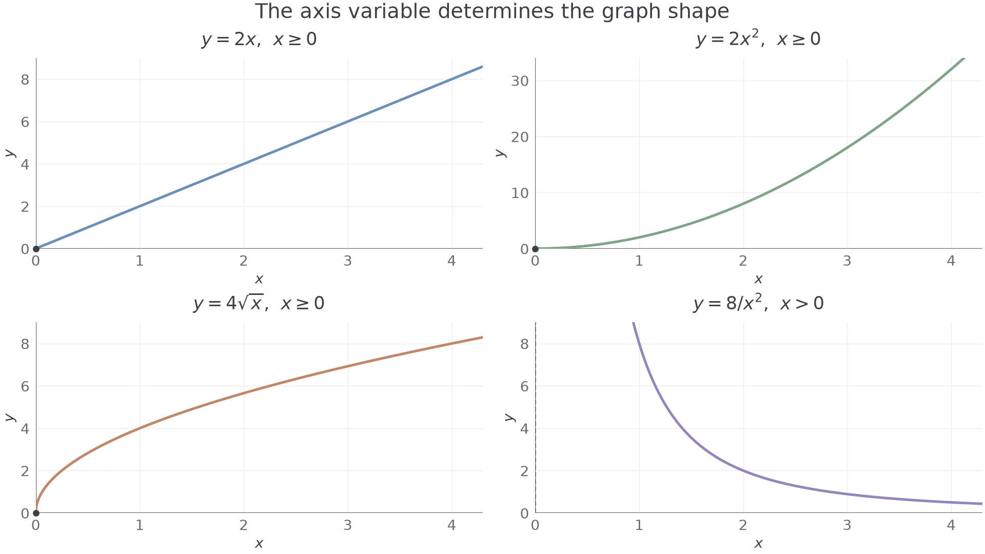
Four direct and inverse proportional relationships on their stated domains

The upper panels are $y=2x$ and $y=2x^2$ ; the lower panels are $y=4\sqrt{x}$ and $y=8/x^2$ . The first three include $x=0$ . The inverse-square curve requires $x>0$ . Plotting $y$ against $x^2$ , rather than $x$ , makes $y=kx^2$ a line through the origin with gradient $k$ ; the same idea works with $\sqrt{x}$ .

Watch out

Wrong: multiplying $x$ by $8$ multiplies $k\sqrt[3]{x}$ by $8$ . Right: the multiplier is $\sqrt[3]{8}=2$ ; the constant does not change.

Now switch to a cube root and use the same two-stage calculation.

Inverse proportion to powers and roots

For an inverse-power model with a positive constant and a positive denominator power, increasing the positive input reduces the output because the relevant product stays constant.

Inverse proportion

$y$ is inversely proportional to an expression $u$ if $y=k/u$ , so $yu=k$ , with $u\ne0$ and fixed nonzero $k$ . For example, $y=8/x^2$ is inverse proportion to $x^2$ , rather than direct proportion to $x$ .

This is the distinction needed for the tank: flow rate multiplied by filling time is the fixed volume. For powers, the same reasoning applies to the whole denominator.

Inverse-power model

For $x>0$ ,

y=\frac{k}{x^n}=kx^{-n},\qquad \frac{y_2}{y_1}=\left(\frac{x_2}{x_1}\right)^{-n}

Here $k\ne0$ . Inverse-square uses $n=2$ ; inverse-square-root uses $n=1/2$ . Zero is excluded. A real inverse-square-root model requires $x>0$ .

Not in the formula sheet: learn it.

Calibrate by multiplying by the denominator. This reverses the division in the model.

Worked example 5: inverse-square change

Question. $y$ is inversely proportional to $x^2$ for $x>0$ . Given $y=5$ at $x=2$ , determine $y$ at $x=4$ .

Plan. Find the constant product $yx^2$ , then divide by the new square.

\begin{aligned} k&=5(2^2)=20 &&\text{calibrate the product}\\ y&=\frac{20}{4^2} &&\text{substitute the new input}\\ &=\frac54 &&\text{simplify} \end{aligned}

Why this step? Doubling $x$ quadruples the denominator, so the output must be divided by four.

Answer. $y=5/4$ .

Check. $2^2(5)=4^2(5/4)=20$ .

Change only the denominator power from a square to a square root. The same input doubling now has a much smaller effect.

Worked example 6: inverse-root change

Question. $y$ is inversely proportional to $\sqrt{x}$ for $x>0$ . Given $y=5$ at $x=2$ , determine the exact value of $y$ at $x=4$ .

Plan. Calibrate $y\sqrt{x}$ , then divide by the new square root.

\begin{aligned} k&=5\sqrt2 &&\text{multiply by the old root}\\ y&=\frac{5\sqrt2}{\sqrt4} &&\text{use the new input}\\ &=\frac{5\sqrt2}{2} &&\text{evaluate the denominator} \end{aligned}

Why this step? It is the root, rather than the input itself, that is in the constant product.

Answer. $y=5\sqrt2/2$ .

Check. The multiplier is $2^{-1/2}=1/\sqrt2$ , so $5/\sqrt2=5\sqrt2/2$ .

For nonzero $k$ , reciprocal and inverse-square graphs have asymptotes $x=0$ and $y=0$ . On a positive physical domain they approach the axes without reaching them. Plotting $y$ against $1/x^2$ or $1/\sqrt{x}$ , as appropriate, produces a line through the origin with gradient $k$ .

Watch out

Wrong: “inversely proportional to $\sqrt{x}$ ” means $y=k\sqrt{x}$ . Right: place the root in the denominator, $y=k/\sqrt{x}$ , and require $x>0$ .

The horizontal-axis label is part of a graph's mathematics. Name the variable, rather than just saying “a straight line”.

Construct and evaluate a proportional model

A model needs more than an equation that fits one pair: its assumptions, domain and predictions must make sense.

For positive observations, compare $y/x$ , $y/x^2$ , $xy$ or $x^2y$ , according to the proposed relationship. For $(1,6)$ , $(2,24)$ and $(3,54)$ , the values of $y/x^2$ are all $6$ , supporting $y=6x^2$ at those inputs. Finite data support a model; they do not prove a law for every input.

Worked example 7: a model survives a check

Question. A fixed empty tank fills at a steady flow rate $q$ litres per second. Assume $T$ , its filling time in seconds, is inversely proportional to $q$ . At $q=3$ , $T=80$ . Determine the model and test it against the observation $T=48$ at $q=5$ .

Plan. Use the first observation to calibrate $T=k/q$ , then compare its prediction with the second observation.

\begin{aligned} k&=80(3)=240 &&\text{fixed volume in litres}\\ T&=\frac{240}{q} &&\text{insert the constant}\\ T(5)&=\frac{240}{5}=48 &&\text{predict independently} \end{aligned}

Why this step? The second observation tests the calibrated equation; using it to change the constant would hide disagreement.

Answer. $T=240/q$ , for $q>0$ . The observation agrees with the prediction.

Check. $3(80)=5(48)=240$ litres. The model assumes a fixed usable volume, steady actual flow and no leaks.

Change only the second measured time from $48$ to $52$ seconds. The calibration stays fixed, so a genuine model check is possible.

Worked example 8: a model misses a measurement

Question. Under the same inverse-proportion assumption, a fixed empty tank takes $80$ seconds at $3$ litres per second. Determine the model and test it against a measured $52$ seconds at $5$ litres per second.

Plan. Calibrate from the first pair and calculate the measured-minus-predicted discrepancy.

\begin{aligned} T&=\frac{80(3)}q=\frac{240}q &&\text{calibrate}\\ T(5)&=48 &&\text{predict}\\ 52-48&=4 &&\text{compare in seconds} \end{aligned}

Why this step? The model predicts the same $240$ -litre volume at every rate, but the second pair gives $5(52)=260$ litres.

Answer. The measured time is $4$ seconds above the prediction. Investigate measurement error or a changing actual flow rate; the discrepancy alone does not identify its cause.

Check. The predicted time decreases as flow increases, as it should. Neither $q=0$ nor unlimited equipment capacity is a sensible model input.

The opening puzzle now has an exact answer: doubling the steady flow from $3$ to $6$ litres per second gives $T=240/6=40$ seconds. A fixed delay before filling, or a pump unable to sustain the quoted rate, would limit that prediction.

Exam tip

When asked to evaluate a model, name an assumption or a specific limitation in this situation. “The model is inaccurate” does not explain what could fail.

Use the same calibration-and-check routine on a different process.

Quick Recap

Direct proportion keeps a ratio constant; inverse proportion keeps a product constant.
A power or root belongs inside the model: $y=kx^n$ and $y=k/x^n$ scale differently.
Read graph axes carefully; plotting against the whole proportional expression produces a line through the origin.
Calibrate, predict and compare with a separate observation, keeping assumptions and domain visible.

Doubling the tank's steady flow halves its filling time: $80$ seconds becomes $40$ seconds, provided the fixed-volume model holds.

Last Accessed

Pure Mathematics

Statistics

Mechanics

1.02r - Proportional relationships and models

Direct proportion and its constant

Proportion to a power or root

Inverse proportion to powers and roots

Construct and evaluate a proportional model

Quick Recap

Learn faster with Nova