2.04a - Finite discrete probability distributions
Use a table or formula to describe a finite discrete random variable, then turn a verbal event into the values you need to add. You will check that a proposed distribution is valid and combine independent observations without losing an order or counting it twice.
A random variable assigns numbers to outcomes
Can two inspections be more likely to find two faults in total than one? Start with one inspection: its fault count is 0, 1 or 2, with probabilities 0.20, 0.50 and 0.30. The most likely single count is 1. That does not yet tell you the most likely total.
You already know
Probabilities lie between 0 and 1. Add probabilities of mutually exclusive events; multiply probabilities of independent events. A complement has probability one minus the event's probability.
The inspection is random, but the rule assigning a number to its outcome is precise.
Finite discrete random variable
A random variable assigns a numerical value to each outcome of a random experiment. A finite discrete random variable has a finite set of possible values, called its support. Write a capital letter such as for the variable and a lower-case for a value. For example, is the fault count; is one possible value. A measurement allowed to take any real value in an interval is not finite discrete.
Here is the complete distribution. Its three events exhaust the possibilities and do not overlap.
| 0 | 1 | 2 | |
|---|---|---|---|
| 0.20 | 0.50 | 0.30 |
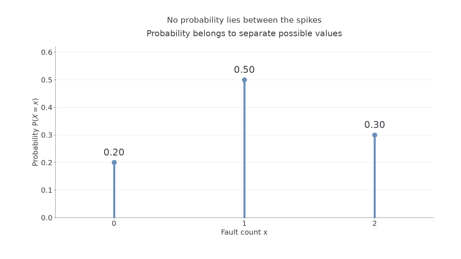
The spike at 1 has height 0.50. There is no spike at 1.5: . A probability table predicts proportions over repetitions; it does not guarantee exact frequencies in a small sample.
Worked example 1: including the endpoint
Question. For this fault-count distribution, find the probability of at most one fault.
Plan. Translate “at most” into an inclusive inequality and add the allowed entries.
Why this step? At most one permits one fault as well as none.
Answer. The probability is 0.70.
Check. Its complement is two faults, with probability 0.30; the probabilities total 1.
Change only whether the endpoint is included. That small wording change removes a whole spike.
Worked example 2: excluding the endpoint
Question. For the same distribution, find the probability of fewer than one fault.
Plan. List the support values strictly below 1.
Why this step? “Fewer than” excludes 1, whose probability is 0.50.
Answer. The probability is 0.20.
Check. The difference from 0.70 is exactly . Also , since the allowed values below 1.5 are 0 and 1.
For an interval, make the same value-by-value decision at both ends.
Watch out
Wrong: . For a discrete variable, the difference is , which can be positive. Read the inequality before touching the calculator.
Try a different complete table; the endpoint is still the key decision.
Probabilities must sum to one
A formula can replace a table, but it needs a stated support and must assign valid probabilities to every value in it.
A valid finite probability distribution
For a finite support ,
The probability is zero outside the support. Not in the formula sheet: learn it.
Use the sum condition to find an unknown constant, then check the individual probabilities. The sum alone cannot rule out negative entries.
Worked example 3: normalising a rule
Question. A variable has for , and zero otherwise. Find and .
Plan. Sum the rule over its complete support, then add the entries for 3 and 4.
Why this step? The support says exactly which terms belong in the normalising sum.
Answer. and the requested probability is 0.70.
Check. The entries 0.1, 0.2, 0.3 and 0.4 are non-negative and total 1; , not .
Keep the rule and the event, but extend the support by one value. The constant must change because the total probability is still 1.
Continue this lesson.
You’re previewing NovaLearn without an account. Create a free account to read the rest.
Create free account