1.03h - Parametric models and restricted parameters | OCR A-Level Mathematics A

Use a shared parameter to connect changing quantities in geometry and motion. You will build equations, translate physical restrictions, and compare predictions with observations while keeping units and timing clear.

Constructing a model with a shared parameter

Can two objects follow exactly the same drawn path yet be in different places one second after they start? A path records positions, but a time parameter also records when they occur. Before exploring that distinction, build a model where the parameter is a length rather than time.

A rectangle with perimeter $20\,\mathrm{cm}$ can have widths $3\,\mathrm{cm}$ and $7\,\mathrm{cm}$ , with heights $7\,\mathrm{cm}$ and $3\,\mathrm{cm}$ . Swapping the sides leaves the area $21\,\mathrm{cm^2}$ unchanged. One shared variable can describe this whole family.

You already know

A parametric point uses one shared parameter value. A physical domain must exclude impossible values, such as negative time after a launch or a non-positive side length.

Define the parameter's meaning and units before writing equations. The letter $t$ does not automatically mean seconds.

Parametric model

A parametric model expresses related quantities through one parameter, with stated meanings, units, assumptions and an allowed domain. The equations and domain together make the prediction.

An ideal geometric constraint can be exact; a model of a real journey also depends on assumptions about how the motion behaves.

Worked example 1: a family of rectangles

Question. A rectangle has perimeter $20\,\mathrm{cm}$ . Use its width $t$ , measured in centimetres, to model width $x$ , height $y$ and area $A$ . Find the area at $t=3$ .

Plan. Use the perimeter constraint and require both sides to be positive.

\begin{aligned} 2x+2y&=20 &&\text{fixed perimeter}\\ x&=t,\quad y=10-t &&\text{shared width parameter}\\ 0&<t<10 &&\text{both lengths positive}\\ A&=t(10-t) &&\text{width times height}\\ A(3)&=3(7)=21 &&\text{substitute} \end{aligned}

Why this step? The boundary values would give flattened shapes, not rectangles with positive side lengths.

Answer. $x=t$ , $y=10-t$ , $A=t(10-t)$ , $0<t<10$ , with $A(3)=21\,\mathrm{cm^2}$ .

Check. At $t=3$ , $2(3)+2(7)=20\,\mathrm{cm}$ .

Change only the perimeter from $20$ to $24\,\mathrm{cm}$ , retaining the width parameter.

Worked example 2: a new fixed perimeter

Question. Build the same model for perimeter $24\,\mathrm{cm}$ , and evaluate its area at $t=3$ .

Plan. Halve the new perimeter to relate the side lengths.

\begin{aligned} x+y&=12 &&\text{halve the perimeter}\\ x&=t,\quad y=12-t &&\text{express both sides}\\ 0&<t<12,\quad A=t(12-t) &&\text{positive sides and area}\\ A(3)&=3(9)=27 &&\text{evaluate} \end{aligned}

Why this step? The allowable width changes with the perimeter; the previous upper limit $10$ no longer describes the full family.

Answer. $x=t$ , $y=12-t$ , $A=t(12-t)$ , $0<t<12$ , with area $27\,\mathrm{cm^2}$ at $t=3$ .

Check. $2(3)+2(9)=24\,\mathrm{cm}$ .

These perimeter and area models are derived from the geometry; they are not in the formula sheet. Increasing width by $1\,\mathrm{cm}$ decreases height by $1\,\mathrm{cm}$ , preserving the perimeter. This is a simple example of quantities whose changes are linked.

Watch out

Wrong: $0\le t\le12$ for a rectangle with positive sides. Right: $0<t<12$ ; the endpoints are degenerate shapes.

Change the perimeter again and use the same modelling decision.

Time, position and average changes

When the parameter is time, coordinate equations retain the timing of a journey. The initial coordinates and coordinate rates play different roles.

Average coordinate rate

For two distinct times $t_1,t_2$ ,

\text{average }x\text{-rate}=\frac{x(t_2)-x(t_1)}{t_2-t_1},\qquad \text{average }y\text{-rate}=\frac{y(t_2)-y(t_1)}{t_2-t_1}.

Use consistent position and time units. Not in the formula sheet: learn it.

For a coordinate that is linear in time, the same rate applies over every permitted interval. A curved coordinate-time graph need not have one constant rate.

Worked example 3: a timed straight path

Question. A boat has position $x=2+3t$ , $y=1+2t$ , $0\le t\le4$ , in metres and seconds. Find its endpoints, average coordinate rates and Cartesian path.

Plan. Substitute the endpoint times, then eliminate $t$ using the $x$ -equation.

\begin{aligned} t=0,4&:\ (2,1),\ (14,9) &&\text{positions}\\ \frac{14-2}{4}&=3,\quad\frac{9-1}{4}=2 &&\text{average rates}\\ t&=\frac{x-2}{3} &&\text{recover time}\\ y&=1+\frac23(x-2),\quad 2\le x\le14 &&\text{path and restriction} \end{aligned}

Why this step? The constants $2$ and $1$ locate the starting point; the coefficients $3$ and $2$ describe coordinate change per second.

Answer. The boat goes from $(2,1)$ to $(14,9)$ , with average coordinate rates $3$ and $2\,\mathrm{m\,s^{-1}}$ ; its path is the stated segment.

Check. At $t=1$ , $(5,3)$ satisfies the Cartesian equation.

Change only the time origin: write $u=t-1$ , still measured in seconds. The journey is unchanged.

Worked example 4: a different clock origin

Question. Express the same boat model in terms of $u=t-1$ , giving its new domain and starting point.

Plan. Substitute $t=u+1$ throughout, including the interval.

\begin{aligned} x&=2+3(u+1)=5+3u &&\text{replace the time variable}\\ y&=1+2(u+1)=3+2u &&\text{same replacement}\\ -1&\le u\le3 &&\text{shift both boundaries} \end{aligned}

Why this step? $u=0$ means the old time $t=1$ , not the beginning of observation.

Answer. $x=5+3u$ , $y=3+2u$ , $-1\le u\le3$ , starting at $(2,1)$ when $u=-1$ .

Check. At $u=3$ , $(x,y)=(14,9)$ , the unchanged final point.

The Cartesian path no longer carries the clock labels. Keep the parameter if the question asks when a point is reached.

Watch out

Wrong: changing to $u=t-1$ means starting the same journey at $u=0$ . Right: translate the domain too; the journey begins at $u=-1$ .

Move the time origin another second.

A projectile path with a physical domain

A supplied flight model can be investigated by algebra before studying its instantaneous velocity. Here $x$ is horizontal distance, $y$ is height, both in metres, and $t$ is seconds after launch. Assume a point object, level ground, constant downward gravitational acceleration and negligible air resistance until landing.

[DIAGRAM: asset_name: A restricted projectile model; caption: A restricted projectile model; asset_slug: h240-projectile-path; description: The path x equals 10t and y equals 9.8t minus 4.9t squared for 0 to 2 seconds, with launch, landing, peak at 10 comma 4.9 and two equal-height positions labelled]

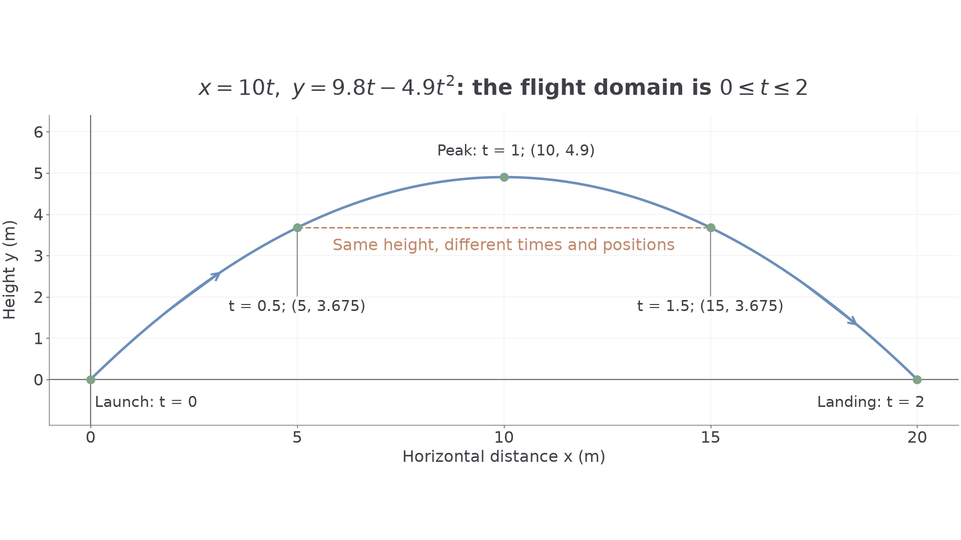
The graph stops at landing. Its algebraic continuation below ground is not part of the airborne journey.

Worked example 5: determine a flight domain

Question. For $x=10t$ , $y=9.8t-4.9t^2$ , find the flight domain, Cartesian path and highest point.

Plan. Solve $y=0$ for landing, eliminate time, then complete the square for the peak.

\begin{aligned} y&=4.9t(2-t)=0 &&\text{ground level}\\ t&=0\text{ or }2 &&\text{launch or landing}\\ y&=0.98x-0.049x^2,\quad 0\le x\le20 &&\text{use }t=x/10\\ y&=4.9-4.9(t-1)^2 &&\text{complete the square} \end{aligned}

Why this step? The positive ground-level root ends the flight; the zero root describes launch.

Answer. $0\le t\le2$ , with the stated Cartesian path. The highest point is $(10,4.9)$ , at $t=1$ .

Check. At $t=0.5$ and $1.5$ , the heights are both $3.675\,\mathrm m$ , but the horizontal positions are $5$ and $15\,\mathrm m$ .

Change only the horizontal coefficient from $10$ to $14$ . The height-time equation and landing time stay fixed.

Worked example 6: change the horizontal motion

Question. For $x=14t$ , $y=9.8t-4.9t^2$ , find the flight domain, Cartesian path and highest point.

Plan. Keep the height analysis and replace the time elimination by $t=x/14$ .

\begin{aligned} 0&\le t\le2 &&\text{unchanged ground roots}\\ y&=9.8\left(\frac{x}{14}\right)-4.9\left(\frac{x}{14}\right)^2 &&\text{eliminate }t\\ &=0.7x-0.025x^2,\quad0\le x\le28 &&\text{simplify and restrict} \end{aligned}

Why this step? Changing horizontal motion stretches the path horizontally but does not change when the height reaches zero.

Answer. The flight lasts $2\,\mathrm s$ , the path is as stated, and the highest point is $(14,4.9)$ , at $t=1$ .

Check. At $x=14$ , $0.7(14)-0.025(14)^2=4.9$ .

The flight equations are supplied models here, not extra recall formulae. The first model's average vertical rates from launch to peak and peak to landing are $4.9$ and $-4.9\,\mathrm{m\,s^{-1}}$ ; its horizontal rate is $10\,\mathrm{m\,s^{-1}}$ throughout. Equal interval averages do not establish constant vertical motion. The derived Cartesian paths are not in the formula sheet.

Watch out

Wrong: use all $t\ge0$ because the equations accept those values. Right: stop at the first landing; later negative heights lie outside this flight model.

Keep the height equation and change the horizontal coefficient again.

Checking a parametric model against observations

A correct calculation does not guarantee that a model matches a real journey. Compare both predicted coordinates with observations at the same recorded time.

Coordinate discrepancy

A coordinate discrepancy is the observed value minus the model's predicted value, with its units and sign. A discrepancy may reflect measurement error or a modelling assumption; one observation alone rarely identifies its cause.

Use the same subtraction order for both coordinates, so a negative value consistently means the observation lies below the prediction in that coordinate.

Worked example 7: compare a flight observation

Question. The model $x=10t$ , $y=9.8t-4.9t^2$ predicts a flight in metres. At $t=1\,\mathrm s$ , the observed position is $(10.3,4.6)$ . Find observed minus predicted and suggest one assumption to investigate.

Plan. Evaluate the model at the observation time, then subtract coordinate by coordinate.

\begin{aligned} (x,y)_{\text{predicted}}&=(10,4.9) &&\text{use }t=1\\ \text{observed}-\text{predicted}&=(10.3-10,\ 4.6-4.9) &&\text{consistent order}\\ &=(0.3,-0.3)\,\mathrm m &&\text{calculate} \end{aligned}

Why this step? Comparing observations with a different time would confuse timing error with position error.

Answer. The discrepancies are $(0.3,-0.3)\,\mathrm m$ . Investigate neglected air resistance or the assumed launch values; measurement uncertainty is another possibility.

Check. Adding the discrepancy to $(10,4.9)$ recovers $(10.3,4.6)$ .

Change only the observation to $(9.8,5.0)$ , keeping the model and time.

Worked example 8: the signs change

Question. Find the discrepancies for this new observation and explain whether they prove that air resistance caused the mismatch.

Plan. Use the same prediction and distinguish a calculated mismatch from evidence of a particular cause.

\begin{aligned} (x,y)_{\text{predicted}}&=(10,4.9) &&\text{unchanged prediction}\\ \text{observed}-\text{predicted}&=(9.8-10,\ 5.0-4.9) &&\text{subtract}\\ &=(-0.2,0.1)\,\mathrm m &&\text{retain the signs} \end{aligned}

Why this step? Many sources can produce one discrepancy, so its existence alone does not identify the cause.

Answer. The discrepancies are $(-0.2,0.1)\,\mathrm m$ . They do not prove an air-resistance explanation; compare further observations and measurement uncertainty.

Check. $(10,4.9)+(-0.2,0.1)=(9.8,5.0)$ .

The opening timing puzzle has a precise example. For $x=2+3t$ , $y=1+2t$ , $0\le t\le4$ , replacing $t$ by $2s$ gives $x=2+6s$ , $y=1+4s$ , $0\le s\le2$ . These describe the same path. If $s=t/2$ is just a new parameter label, they describe the same journey. If both letters are claimed to be actual elapsed seconds, at one second they predict $(5,3)$ and $(8,5)$ : different journeys. This timing comparison is not a formula-sheet result.

Key idea

A Cartesian path says where a point can be; a time parametrisation also says when. Check observations against both coordinates at the stated time.

Use a fresh observation to test the flight model without claiming more than the data show.

Quick Recap

Define what the parameter means, its units and its permitted values.
Translate geometric and physical constraints into parameter restrictions.
Eliminate time to describe a path, but retain time equations for timing questions.
Stop a flight model at landing and distinguish launch and landing roots.
Compare observations at the same parameter value and investigate assumptions without claiming a unique cause from one discrepancy.

Yes: the opening objects can share a path but have different timings. The models with coordinate rates $(3,2)$ and $(6,4)$ trace the same segment at different rates when their parameters both represent elapsed seconds.

Last Accessed

Pure Mathematics

Statistics

Mechanics

1.03h - Parametric models and restricted parameters

Constructing a model with a shared parameter

Time, position and average changes

A projectile path with a physical domain

Checking a parametric model against observations

Quick Recap

Learn faster with Nova