1.03c - Straight line models and rates of change | OCR A-Level Mathematics A

Build straight-line models from constant-change assumptions and observations. You will interpret rates and intercepts with their units, choose sensible domains and time origins, and test predictions against further evidence.

Constant change and model assumptions

A tank holds $400$ litres, then $280$ litres after $8$ minutes. Can two observations tell you when it will be empty? They can give a prediction, but only after you choose an assumption about what happens between and beyond them.

You already know

A line has equation $y=mx+c$ . Its gradient is change in output divided by change in input; its intercept is the output at input zero.

A constant rate makes equal input steps produce equal output changes. That is the reason to choose a line, rather than merely a convenient shape to draw.

Linear model

A linear model represents a relationship by a straight-line equation, usually $y=mx+c$ . The gradient $m$ is the assumed constant rate of change; $c$ is the model's value when $x=0$ . The variables, units, domain and assumptions are part of the model.

A pricing rule can be exactly linear over its stated range. A line fitted to measurements is normally an approximation; two observations alone do not establish constant change.

Worked example 1: a fixed charge and a rate

Question. A delivery booking costs £ $12$ , plus £ $0.80$ per parcel, for at most $40$ parcels. Form a cost model and interpret its constants. A booking with no parcels still incurs the booking fee.

Plan. Separate the fixed charge from the charge that grows with parcel count.

\begin{aligned} \text{variable charge}&=0.80n && \text{rate times count} \\ C&=12+0.80n && \text{add the booking fee} \\ C(10)&=12+8=20 && \text{check one booking} \end{aligned}

Why is $n$ an integer? A booking cannot contain a fraction of a parcel.

Answer. $C=12+0.80n$ , with $C$ in pounds and integer $0\le n\le40$ . The intercept is £ $12$ ; the rate is £ $0.80$ per parcel. This assumes no discounts or extra charges within the range.

Check. Increasing $n$ from $10$ to $11$ changes the cost from £ $20$ to £ $20.80$ , exactly £ $0.80$ .

Change only the fixed booking fee to zero. The rate and allowed parcel counts stay the same.

Worked example 2: a line through the origin

Question. The same service removes its booking fee and retains the rate £ $0.80$ per parcel, for integer $0\le n\le40$ . Form and interpret the model.

Plan. Set the fixed part to zero while retaining the variable part.

\begin{aligned} C&=0+0.80n && \text{no booking charge} \\ C(10)&=8 && \text{substitute a parcel count} \\ C(0)&=0 && \text{evaluate at zero} \end{aligned}

Why does this line pass through the origin? With no fixed fee, zero parcels cost zero.

Answer. $C=0.80n$ pounds. The gradient is still £ $0.80$ per parcel and the intercept is $0$ .

Check. Ten parcels cost £ $8$ , while twenty cost £ $16$ ; doubling the count doubles the whole cost in this model.

With a fixed charge, doubling the count does not double the whole bill: $C(20)=28$ , whereas $2C(10)=40$ in Worked example 1. A straight line need not represent direct proportion. None of these contextual models is in the formula sheet: construct them from the information.

Watch out

Wrong: the gradient is “£ $0.80$ ”. Right: it is £ $0.80$ per parcel. A rate needs both the output and input units.

Interpret a new fixed charge and rate without assuming every straight line passes through the origin.

Constructing a model from two observations

Return to the tank. Assume a constant net loss of water: that makes volume a linear function of elapsed time. A decreasing volume has a negative gradient, while the volume itself stays non-negative.

A model from two observations

For observations $(t_1,V_1)$ , $(t_2,V_2)$ , with $t_1\ne t_2$ , a constant-rate model is

m=\frac{V_2-V_1}{t_2-t_1},\qquad V-V_1=m(t-t_1)

This constructs a model; it does not prove the constant-rate assumption.

Not in the formula sheet: learn it.

Write down what the clock measures before finding the intercept.

Worked example 3: predicting an emptying time

Question. A tank holds $400$ litres at $t=0$ and $280$ litres at $t=8$ , where $t$ is time in minutes. Assume constant net loss. Find the model and predicted emptying time.

Plan. Find the rate, use the initial volume, then set volume equal to zero.

\begin{aligned} m&=\frac{280-400}{8-0}=-15 && \text{litres per minute} \\ V&=400-15t && \text{use the initial value} \\ 0&=400-15t && \text{empty means zero volume} \\ t&=\frac{80}{3} && \text{solve} \end{aligned}

Why set $V=0$ , rather than the gradient to zero? Emptying is a value of the volume; the model's rate stays $-15$ .

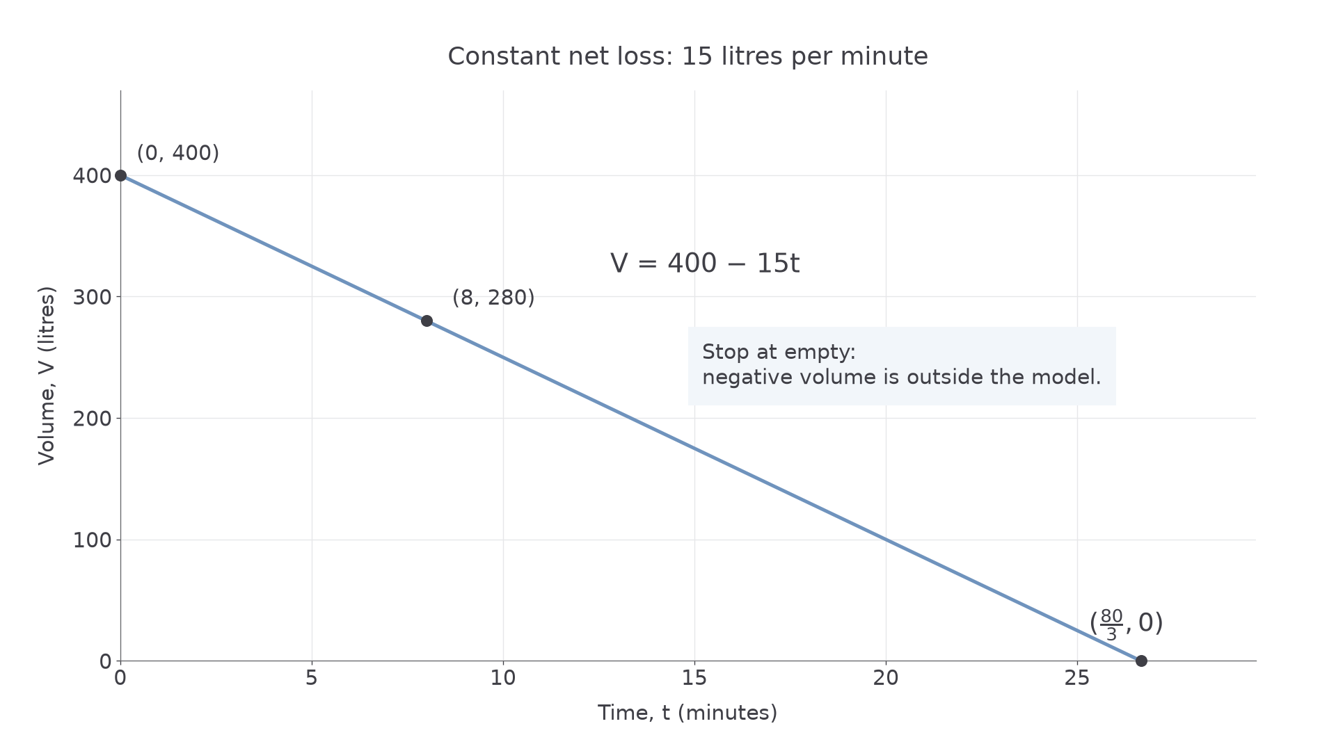
Answer. $V=400-15t$ , with $0\le t\le\frac{80}{3}$ . Emptying is predicted after $\frac{80}{3}$ minutes, provided the loss remains constant.

Check. $V(8)=280$ , $V(12)=220$ , and $400-15(\frac{80}{3})=0$ .

Change only the clock origin: the same two readings are now at $t=2$ and $t=10$ . The elapsed time between them stays $8$ minutes.

Worked example 4: observations away from zero

Question. A tank holds $400$ litres at clock reading $t=2$ minutes and $280$ litres at $t=10$ . Assume the same constant loss continues. Find its model and the clock reading at emptying.

Plan. Use the rate and an observed point, rather than treating $400$ as the intercept.

\begin{aligned} m&=\frac{280-400}{10-2}=-15 && \text{rate is unchanged} \\ V-400&=-15(t-2) && \text{use the first observation} \\ V&=430-15t && \text{expand} \\ 0=430-15t&\Rightarrow t=\frac{86}{3} && \text{solve for emptying} \end{aligned}

Why is the intercept now $430$ ? The clock's zero is two minutes before the first reading, so the constant-rate extension adds $30$ litres.

Answer. $V=430-15t$ ; emptying is predicted at $t=\frac{86}{3}$ minutes. From the first reading, the elapsed time is still $\frac{80}{3}$ minutes.

Check. $430-15(2)=400$ and $430-15(10)=280$ .

[DIAGRAM: asset_name: Constant water loss with a physical endpoint; caption: The constant-rate tank model stops at zero volume; asset_slug: h240-tank-model; description: A volume-time graph shows V equals 400 minus 15t from t equals zero to 80 over 3 minutes, through the observed points 0 comma 400 and 8 comma 280. The segment ends at empty, rather than extending into negative volumes. Axes show minutes and litres.]
The constant-rate tank model stops at zero volume

For a pricing example with neither input zero, journeys of $10$ km for £ $23$ and $30$ km for £ $35$ give rate $(35-23)/(30-10)=0.60$ pounds per kilometre. Hence $C-23=0.60(d-10)$ , or $C=17+0.60d$ . Interpreting £ $17$ as an actual zero-distance charge needs the tariff to apply there too.

Watch out

Wrong: extend the tank line past emptying and interpret a negative prediction as water remaining. Right: state the physical domain and stop the volume model at zero.

Use a new pair of nonzero-time readings. The emptying time is a conditional prediction, not another observation.

Average rates and the choice of origin

An average rate uses total change over an interval. The quantity may rise and fall within that interval: the endpoints alone do not tell you its rate at each moment.

Average rate of change

The average rate of change is total output change divided by total input change over a nonzero interval. Its units are output units per input unit. It equals the gradient of the line joining the two observations.

Changing the clock origin changes an intercept without changing that rate. In fact, substituting $t=u+a$ into $Y=mt+c$ gives $Y=mu+(ma+c)$ : the same physical process can have different intercepts simply because the clock was reset. This identity is not in the formula sheet; it follows by substitution.

Worked example 5: hours after midnight

Question. A temperature is $18^\circ\mathrm C$ at 09:00 and $24^\circ\mathrm C$ at 13:00. Find its average rate and a constant-rate model, using $t$ hours after midnight.

Plan. Divide the temperature change by four hours, then use the observation at $t=9$ .

\begin{aligned} m&=\frac{24-18}{13-9}=1.5 && \text{degrees Celsius per hour} \\ T-18&=1.5(t-9) && \text{use the first reading} \\ T&=1.5t+4.5 && \text{expand} \end{aligned}

Why is the first time $9$ , not $0$ ? This clock counts hours after midnight.

Answer. Average rate $1.5^\circ\mathrm{C}$ per hour; model $T=1.5t+4.5$ , $9\le t\le13$ . The intercept is an algebraic extension to midnight, not a measured midnight temperature.

Check. At 11:00, the model gives $T=21^\circ\mathrm C$ , halfway between the two readings.

Change only the time origin to 09:00. The temperatures and physical interval stay fixed.

Worked example 6: hours after the first observation

Question. Model the same readings using $u$ , hours after 09:00.

Plan. Substitute $t=u+9$ into the existing model.

\begin{aligned} T&=1.5(u+9)+4.5 && \text{change the time variable} \\ T&=18+1.5u && \text{collect constants} \end{aligned}

Why does the intercept become $18$ ? The new zero is exactly the first observation.

Answer. $T=18+1.5u$ , with $0\le u\le4$ ; the rate is unchanged.

Check. At 11:00, $u=2$ , so $T=18+3=21^\circ\mathrm C$ , as before.

Neither line proves the temperature increased steadily. It might have dipped and then recovered; using a constant-rate model adds an assumption to the measured average.

Watch out

Wrong: the average rate is $4/6$ hours per degree. Right: temperature change divided by elapsed time gives $6/4=1.5$ degrees per hour.

State both the variable's origin and its interval in the next model.

Checking and refining a linear model

A model becomes more useful when you test it on information that did not construct it. Calculate a discrepancy first, then discuss what it suggests; an error alone does not identify its cause.

Interpolation and extrapolation

Interpolation predicts within the observed input range. Extrapolation predicts beyond it. Extrapolation relies more heavily on the relationship continuing outside the available evidence; neither process guarantees an accurate prediction.

For a numerical comparison, define the signed discrepancy as observed minus predicted. This definition is not a formula-sheet result; stating the order prevents a sign from losing its meaning.

Worked example 7: an observation above the model

Question. A journey-price model $C=17+0.60d$ was fitted to distances $10$ km and $30$ km. A separate $20$ km journey costs £ $32$ . Calculate observed minus predicted and discuss the discrepancy.

Plan. Predict at the observed distance, subtract in the stated order, then interpret.

\begin{aligned} C(20)&=17+0.60(20)=29 && \text{model prediction} \\ \text{observed minus predicted}&=32-29=3 && \text{signed discrepancy} \end{aligned}

Why compare at the same distance? A price difference is meaningful only for the same input.

Answer. The observation is £ $3$ above the prediction. An extra charge or a changing tariff could explain it, but further information is needed. This is interpolation because $10<20<30$ .

Check. £ $29$ +£ $3$ =£ $32$ .

Change only the new observed cost, from £ $32$ to £ $28$ .

Worked example 8: an observation below the model

Question. For the same model and fitted range, a separate $20$ km journey costs £ $28$ . Calculate observed minus predicted and interpret it.

Plan. Keep the prediction fixed and update the observed value.

\begin{aligned} C(20)&=29 && \text{same model and input} \\ \text{observed minus predicted}&=28-29=-1 && \text{subtract in the stated order} \end{aligned}

Why retain the negative sign? It tells you the model overpredicts the observed charge.

Answer. The observation is £ $1$ below the model. A discount could be relevant, but the discrepancy alone does not establish that explanation.

Check. The model prediction exceeds the observation by £ $1$ , consistent with the negative discrepancy.

A $60$ km prediction would extrapolate beyond the fitted range. Collect further observations and check the tariff before relying on it. A known discount boundary may require two linear pieces; a steadily changing rate may require a curved model. Compare errors across observations rather than forcing the line through one extra point and declaring the problem solved.

Exam tip

Explain a limitation in the context: “the constant loss rate may change as the battery usage changes” says more than “the model is inaccurate”. Keep a discrepancy in percentage points distinct from a percentage change.

The tank's predicted emptying time has the same limitation: a constant net loss must continue all the way to empty.

Quick Recap

State variables, units, domains and the assumption of constant change.
Gradient is a rate; the intercept belongs to the chosen input zero.
Two observations determine a proposed line, rather than prove a constant rate.
Changing the time origin changes the intercept but leaves the gradient unchanged.
Check further observations and physical limits before trusting a prediction.

The opening tank is predicted to empty after $\frac{80}{3}$ minutes under $V=400-15t$ ; that conclusion depends on the net loss remaining constant.

Last Accessed

Pure Mathematics

Statistics

Mechanics

1.03c - Straight line models and rates of change

Constant change and model assumptions

Constructing a model from two observations

Average rates and the choice of origin

Checking and refining a linear model

Quick Recap

Learn faster with Nova