2.02c–2.02e - Scatter diagrams, regression and correlation
Interpret paired data and supplied regression lines in 2.02c, describe correlation informally in 2.02d, and distinguish association from cause in 2.02e. You will see how a convincing overall trend can hide the opposite pattern within each group.
Reading relationships in paired data
Can longer cycle journeys look quicker overall, although longer journeys take more time within each route type? A hill route and a flat route can create exactly that puzzle.
You already know
A point means one journey of distance and time . Coordinate order and units matter.
A scatter diagram preserves two measurements from the same person, object or event. Sorting the two columns independently destroys those pairings and can manufacture a relationship.
Bivariate data and correlation
Bivariate data contain two variables for each observational unit. An association is a relationship between them. Positive correlation means larger values of one tend to accompany larger values of the other; negative correlation means larger values tend to accompany smaller ones. Strong linear correlation has points close to a straight line; weak linear correlation has more scatter around that trend.
A shallow, tightly aligned cloud can have stronger correlation than a steep, diffuse cloud. Converting kilometres to metres changes a gradient without changing how tightly the points follow a line. Describe the tendency in context: “Longer journeys tend to take more time”, rather than claiming every longer journey takes longer.
A curved relationship can be strong even when there is little linear correlation. No apparent pattern in a sample does not prove that population variables are independent. Here you judge correlation by eye; numerical coefficients and their tests come later.
Key idea
Direction describes whether the cloud rises or falls; strength describes its scatter around a linear trend. Gradient is not a measure of strength.
Look for both features, rather than treating any downward trend as automatically strong.
Subgroups and unusual paired observations
A pooled cloud can combine different sections of a population whose separate patterns tell a different story.
The left panel uses constructed cycle-commute data. Hill-route journeys are shorter but generally slower; flat-route journeys are longer but generally quicker. Within either route type, increasing distance is accompanied by increasing time. The reversal on pooling is a real mathematical possibility, not an error in reading the axes.
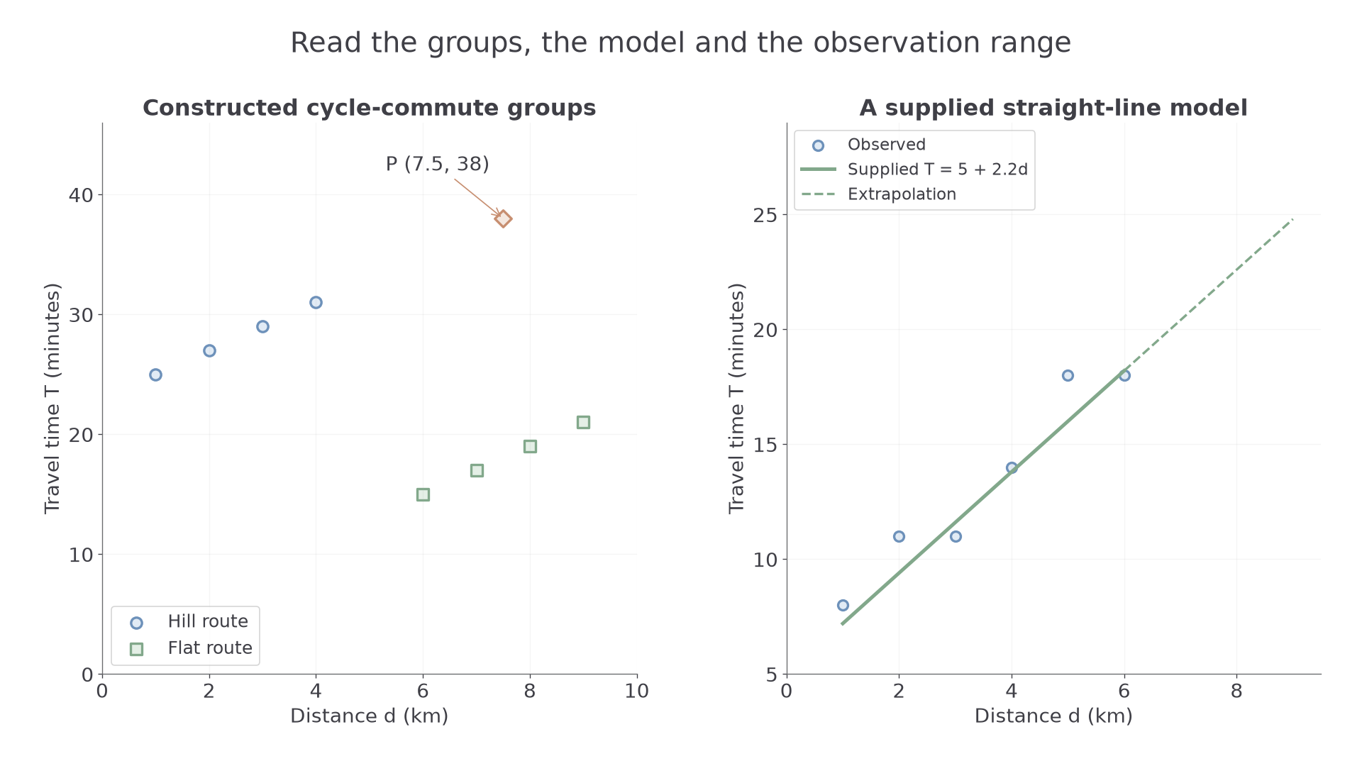
Point P at is inconsistent with nearby flat-route observations. It might reflect a stop, different conditions or a recording error. Investigate its source rather than deleting it simply because it changes the pattern. A point far along the distance axis is not automatically unusual if it follows the relevant trend.
Worked example 1: two separate relationships
Question. A constructed sample has urban journeys and rural journeys , with distance in km and time in minutes. Describe the within-group and between-group relationships.
Plan. Compare changes within each group before comparing the two groups.
Why separate the groups? Route conditions change at the same time as the distance range.
Answer. Time increases with distance within both groups. Rural journeys are longer but all have shorter times here, so one pooled description can hide the positive within-group relationships.
Check. The third point of each group also increases by 3 minutes for the next kilometre.
Change only the rural group's times by adding 15 minutes to each. Within-group changes remain fixed.
Worked example 2: changing the separation between groups
Question. Keep the urban points above, but take rural points . Describe the within-group and between-group relationships.
Plan. Recheck both levels of the comparison after the vertical shift.
Why does the overall impression change? Shifting a whole group alters the pooled cloud while preserving that group's internal trend.
Answer. Both groups still show increasing time with distance, and the longer rural journeys are now slower than the urban journeys. The pooled and within-group directions now agree.
Check. Every rural time rose by exactly 15 minutes; none of the rural time differences changed.
In a supplied diagram, an additional point belongs at distance 4 and time 14 on the existing axes. A vertical boundary around separates the two pictured route groups; a boundary through a cluster would split that group. You may be asked to make such additions, but are not required to draw a complete scatter diagram or calculate a regression equation.
Watch out
Wrong: “The pooled cloud falls, so increasing distance makes each cyclist faster.” The groups may differ in route conditions. Inspect groups before interpreting an overall association.
Try one more vertical shift with fresh values.
Continue this lesson.
You’re previewing NovaLearn without an account. Create a free account to read the rest.
Create free account