2.05d, 2.05e - The sample mean and normal mean tests | OCR A-Level Mathematics A

Why can a small change in an average be convincing when individual measurements vary widely? Treat a sample mean as a random variable, then test a normal population's mean using a known, given or assumed population variance.

The distribution of a sample mean

Could a sample mean of $52.1$ ml provide evidence against a claimed mean fill of $50$ ml when individual fills have standard deviation $8$ ml? The key is that averages vary less than individual observations.

You already know

In $X\sim\mathrm N(\mu,\sigma^2)$ , the second parameter is the variance. Standardise an individual value by subtracting its mean and dividing by its standard deviation.

Before taking a random sample, its mean is unknown and random. Once the measurements are observed, that random quantity has a particular numerical value.

Sample mean

For an independent random sample $X_1,\ldots,X_n$ , the sample mean is the random variable $\bar X=(X_1+\cdots+X_n)/n$ . Its observed value is $\bar x$ . The population mean $\mu$ is a fixed parameter; it is neither the sample mean random variable nor its observed value.

For a normal population the following distribution is exact, even for a small independent random sample. Use the result without proving it.

Distribution of the sample mean

If observations come independently from $X\sim\mathrm N(\mu,\sigma^2)$ , then

\bar X\sim\mathrm N\!\left(\mu,\frac{\sigma^2}{n}\right),\qquad \frac{\bar X-\mu}{\sigma/\sqrt n}\sim\mathrm N(0,1).

The standard deviation of $\bar X$ , called its standard error, is $\sigma/\sqrt n$ .

In the formula sheet.

Quadrupling the sample size only halves the standard error. An average of one hundred independent measurements has one tenth the standard deviation of one measurement, rather than one hundredth.

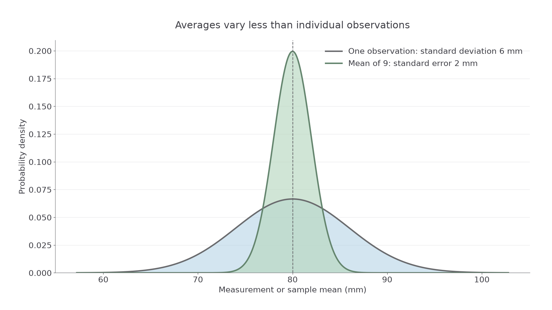
Normal distributions for individual lengths and means of nine independent lengths

Both distributions have mean $80$ mm; the sample means are much less spread out.

Worked example 1: a probability for an average

Question. Component lengths in millimetres follow $\mathrm N(80,36)$ . For an independent random sample of nine, find $\mathrm P(\bar X>83)$ .

Plan. Find the variance and standard error of the mean before standardising.

\begin{aligned} \bar X&\sim\mathrm N(80,36/9)=\mathrm N(80,4)\\ \mathrm{SE}&=\sqrt4=2\\ \mathrm P(\bar X>83)&=\mathrm P\!\left(Z>\frac{83-80}{2}\right)\\ &=\mathrm P(Z>1.5)=0.0668072\ldots \end{aligned}

Why this step? The question concerns an average, so divide the population variance by nine before taking the square root.

Answer. The probability is $0.0668$ , to $3$ significant figures.

Check. The boundary is $1.5$ standard errors above the mean, so an upper-tail probability below $0.5$ is sensible.

Change only the sample size from nine to thirty-six. The population and the boundary stay fixed.

Worked example 2: a larger sample

Question. Find $\mathrm P(\bar X>83)$ for thirty-six independent components from the same population.

Plan. Update the sample-mean variance and repeat the same standardisation.

\begin{aligned} \bar X&\sim\mathrm N(80,36/36)=\mathrm N(80,1)\\ \mathrm P(\bar X>83)&=\mathrm P(Z>3)=0.001349898\ldots \end{aligned}

Why this step? Quadrupling the sample size halves the standard error, so the same $3$ mm departure is now twice as many standard errors away.

Answer. The probability is $0.00135$ , to $3$ significant figures.

Check. Averages from larger samples cluster more tightly around $80$ ; exceeding $83$ becomes less likely.

The distribution applies to independent sampling. Repeated readings from the same unusually long component are not automatically independent components.

Watch out

The sample-mean variance is $\sigma^2/n$ , but its standard deviation is $\sigma/\sqrt n$ . Using $\sigma/n$ makes the distribution far too narrow.

Use the same reasoning for another measurement.

Setting up and carrying out a mean test

A mean test asks whether the observed average is unusually far in the proposed direction from a claimed population mean.

Define $\mu$ as the population mean of the named quantity. Write $\mathrm H_0:\mu=\mu_0$ , with $\mathrm H_1:\mu>\mu_0$ for an increase, $\mu<\mu_0$ for a decrease, or $\mu\ne\mu_0$ for any change. Use a normal population with known, given or assumed variance; do not estimate that variance from the sample for this test.

Standardised mean under the null

For independent normal observations with population standard deviation $\sigma$ , under $\mathrm H_0:\mu=\mu_0$ ,

\bar X\sim\mathrm N\!\left(\mu_0,\frac{\sigma^2}{n}\right),\qquad z=\frac{\bar x-\mu_0}{\sigma/\sqrt n}.

In the formula sheet.

For an upper-tail alternative use $\mathrm P(Z\ge z)$ ; for a lower-tail alternative use $\mathrm P(Z\le z)$ . These tail-choice rules are not printed in the sheet: learn them. Compare the probability with the preselected level, then conclude about the population mean in context.

Worked example 3: the fill-volume question

Question. Fills are normally distributed with given population standard deviation $8$ ml. A random sample of $64$ has mean $52.1$ ml. Test for an increase from a claimed population mean of $50$ ml at $5\%$ .

Plan. Let $\mu$ be the population mean fill in ml. Use the null centre and the standard error of the average.

\begin{aligned} \mathrm H_0&:\mu=50,\qquad \mathrm H_1:\mu>50\\ \bar X\mid\mathrm H_0&\sim\mathrm N(50,64/64)=\mathrm N(50,1)\\ z&=\frac{52.1-50}{1}=2.1\\ \mathrm P(Z\ge2.1)&=0.0178644\ldots<0.05 \end{aligned}

Why this step? The standard error is $1$ ml, so $2.1$ ml is a substantial departure for an average even though it is small beside an individual's $8$ ml standard deviation.

Answer. Reject $\mathrm H_0$ . There is sufficient evidence at $5\%$ to suggest that the population mean fill exceeds $50$ ml.

Check. The sample mean is on the increasing side of the claim, matching the chosen upper tail.

Change only the observed mean to $51.4$ ml; the model and planned test remain fixed.

Worked example 4: an average within ordinary variation

Question. What conclusion follows for a sample mean of $51.4$ ml in the same experiment?

Plan. Recalculate the standardised observation using the same standard error.

z=\frac{51.4-50}{1}=1.4,\qquad \mathrm P(Z\ge1.4)=0.0807567\ldots>0.05.

Why this step? A mean closer to the null centre has a larger upper-tail probability and gives weaker evidence for an increase.

Answer. Do not reject $\mathrm H_0$ . There is insufficient evidence at $5\%$ to suggest that the population mean fill exceeds $50$ ml.

Check. The standard error remains $1$ , because neither the variance nor sample size changed.

A decrease uses the same model but the lower tail. Calculator inputs should be the null mean and the sample-mean standard deviation, not the observed mean and individual standard deviation.

Watch out

Centring the null distribution at $\bar x$ makes the observation look central by construction. Its centre is $\mu_0$ ; $\bar x$ is the value whose extremeness you assess.

Try a lower-tail test with the population parameter already defined.

Continue this lesson.

You’re previewing NovaLearn without an account. Create a free account to read the rest.

Create free account

Last Accessed

Pure Mathematics

Statistics

Mechanics

2.05d, 2.05e - The sample mean and normal mean tests

The distribution of a sample mean

Setting up and carrying out a mean test

Continue this lesson.

Learn faster with Nova