2.05f, 2.05g - Correlation coefficients and significance tests
A scatter diagram can look convincing without settling what happens in the population. Under 2.05f you will interpret Pearson's coefficient; under 2.05g you will use supplied critical values and p-values to test population linear correlation, then explain what the evidence does and does not establish.
Reading Pearson's correlation coefficient
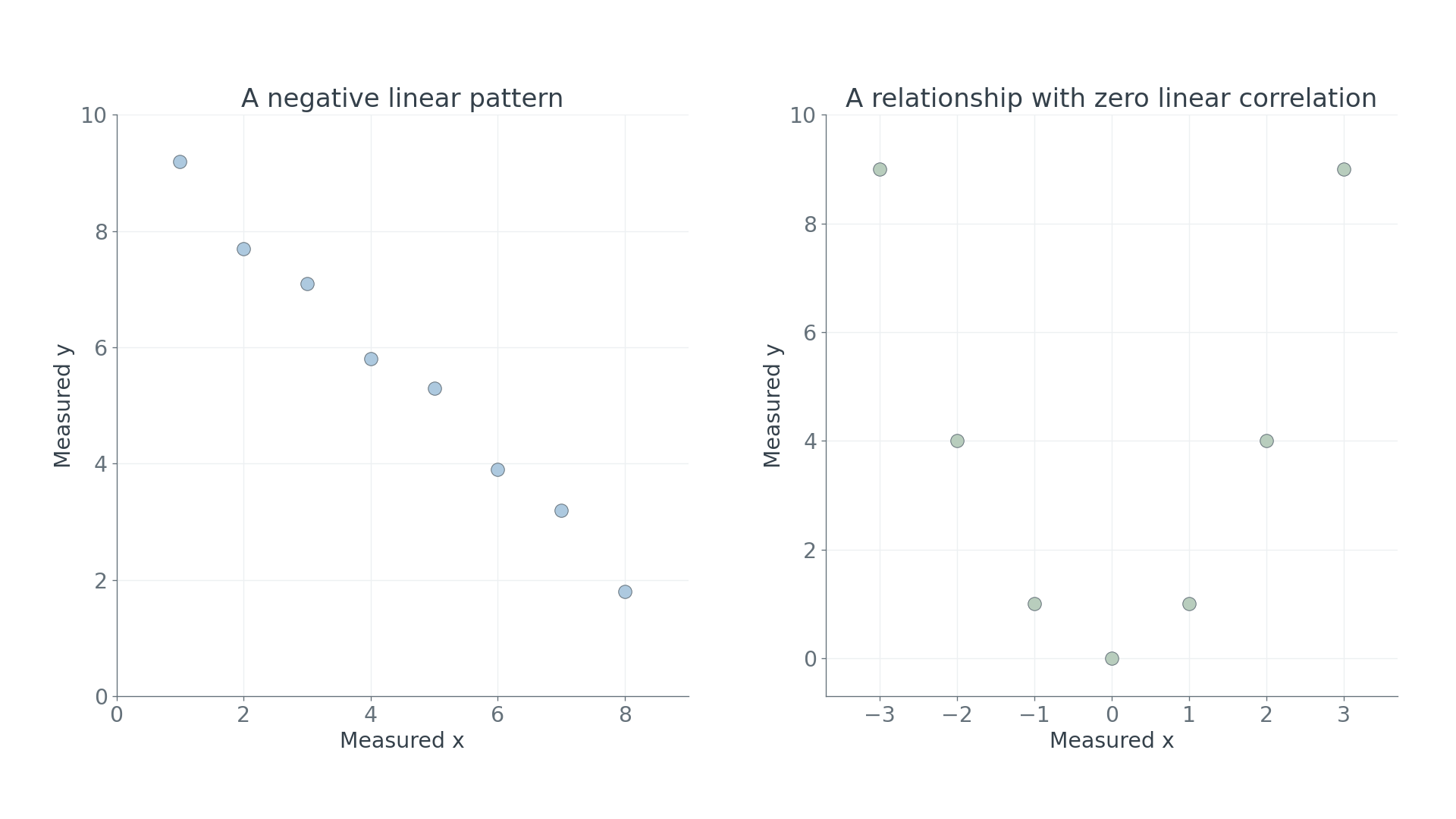
Can two quantities follow an exact rule and still have correlation zero? Take the seven pairs with and . Every height is completely determined by its horizontal position, yet the supplied Pearson coefficient is . A straight-line summary can miss a perfect curve.
You already know
A scatter diagram plots one point for each paired observation. A positive linear pattern rises from left to right; a negative one falls. Correlation alone does not identify a cause.
Compare the curve with the downward pattern. The important question is closeness to a straight line, rather than whether the points fit inside a small patch of the page.
Pearson's product-moment correlation coefficient
The sample Pearson coefficient, , measures the strength and direction of a linear relationship between two varying numerical quantities. It satisfies . Its sign gives the direction; a magnitude closer to indicates points closer to a straight line.
For example, describes points close to a downward-sloping line. A value describes little linear correlation. There are no universal cut-offs that turn every context into the same “strong” or “weak” category. Describe the diagram as well as the number.
Perfect positive linear correlation is , including when all the points lie on . The coefficient is , not the gradient . A coefficient is dimensionless; changing metres to centimetres does not change its magnitude. Perfect negative linear correlation is . If either variable is constant, the usual coefficient is undefined.
These coefficient properties are not in the formula sheet: learn them. You interpret a supplied value here; calculation of correlation coefficients is excluded. Software can supply coefficients during data exploration: retain the paired rows and inspect the scatter diagram before trusting its summary. An outlier or separate groups can alter the coefficient substantially.
Key idea
Zero Pearson correlation means no linear correlation. It does not mean that no relationship exists: the exact U-shaped rule is a counterexample.
Here is a tempting interpretation of another supplied coefficient. Decide which conclusion the number actually supports.
From sample correlation to population hypotheses
A sample can have nonzero correlation just through random variation, so a population claim needs a hypothesis test.
You already know
The null hypothesis gives the population model to test. The alternative describes the departure being investigated. A significance level is a decision threshold chosen before looking at the sample result.
Write for the population Pearson correlation and for the supplied sample coefficient. The observed is already known; is the unknown population parameter.
Population correlation hypotheses
For a test of no population linear correlation,
Choose the alternative from the research question:
Define in context. Not in the formula sheet: learn it.
For the Pearson test, the paired observations may be assumed to come from a bivariate normal distribution, a joint distribution for the two random variables together. State this assumption when asked. Saying merely that each variable separately is normal does not fully state it. A random sample with independent pairs supplies the sampling basis for the test. A scatter diagram can reveal concerns, but cannot prove the joint model.
Worked example 1: a positive claim
Question. A researcher investigates whether taller mature trees tend to have wider canopies. Define a population parameter, state the hypotheses and give the distributional assumption for a Pearson test on an independent random sample of trees.
Plan. Identify the population relationship, translate “wider as height increases” into the alternative, then state the joint model.
Why this step? The question concerns all mature trees in the defined population, rather than whether an observed sample coefficient happens to equal zero.
Answer. Use these hypotheses and assume that the height–canopy-width pairs come from a bivariate normal distribution.
Check. The alternative would be contradicted in direction by a negative sample coefficient, however large its magnitude.
Change only the research claim to a negative one for the same variables and sampling design. The distributional assumption stays the same; the tail changes.
Worked example 2: a negative claim
Question. For the same population and sampling design, a different pre-stated claim is that taller trees tend to have narrower canopies. Define the parameter, state the hypotheses and give the distributional assumption.
Plan. Retain the population parameter and null; reverse only the direction of the alternative.
Why this step? The claim chooses the tail before the data arrive. The sign of the sample cannot retrospectively choose the most favourable alternative.
Answer. Use the negative one-tailed test, assuming a bivariate normal distribution for the paired measurements.
Check. If the question asked whether there was linear correlation in either direction, the alternative would instead be .
Your hypothesis notation must distinguish the population from the sample.
Watch out
Wrong: . The sample value is already observed. Right: , with defined as the population correlation between the named quantities.
The next claim removes the direction. Keep that distinction when you state the alternative.
Using critical values and p-values
A critical value marks the sample results that would be sufficiently unusual under the null hypothesis in the direction of the alternative.
The table supplied with a question is specific to the coefficient and the number of paired observations. A sample of twelve trees means twelve pairs, not twenty-four separate values. Select the significance level and the correct one- or two-tailed heading.
Pearson rejection rules
For a supplied positive critical magnitude , reject when
Use the stated boundary convention in the supplied critical-value table. These rules are not printed on the formula sheet. Not in the formula sheet: learn it.
A p-value offers another route to the same decision.
Continue this lesson.
You’re previewing NovaLearn without an account. Create a free account to read the rest.
Create free account