2.04e–2.04g - Normal models, standardisation and inverse probabilities
Use the mean and variance to interpret a normal model (2.04e), calculate probabilities and inverse boundaries (2.04f), and connect its curve with histograms, spread and familiar proportions (2.04g). The aim is to turn a measurement question into the right area, rather than trust an unexplained calculator output.
The mean centres the curve and the standard deviation sets its spread
A machine cuts rods with mean length 50 mm and standard deviation 4 mm. Under a normal model, what proportion exceed 56 mm? Six millimetres sounds small, but its significance depends on the spread: it is one and a half standard deviations above the mean.
You already know
Variance is the square of standard deviation. In a density histogram, area represents frequency; after scaling the total area to 1, it represents observed proportions. A model describes chance behaviour rather than guaranteeing a sample's exact frequencies.
The curve packages an entire distribution of measurements into a centre and spread.
Normal distribution
A normal distribution is a continuous, symmetric, bell-shaped probability model. In , is the mean and the variance, with . Its symmetry line is ; its inflection points, where the curve changes between convex and concave, lie at .
For lengths in millimetres, the rod model is . Its standard deviation is 4 mm, not 16 mm. The inflections are at 46 and 54 mm. The total area is 1; area between bounds gives their probability, whereas the curve's height is a density, not a probability.
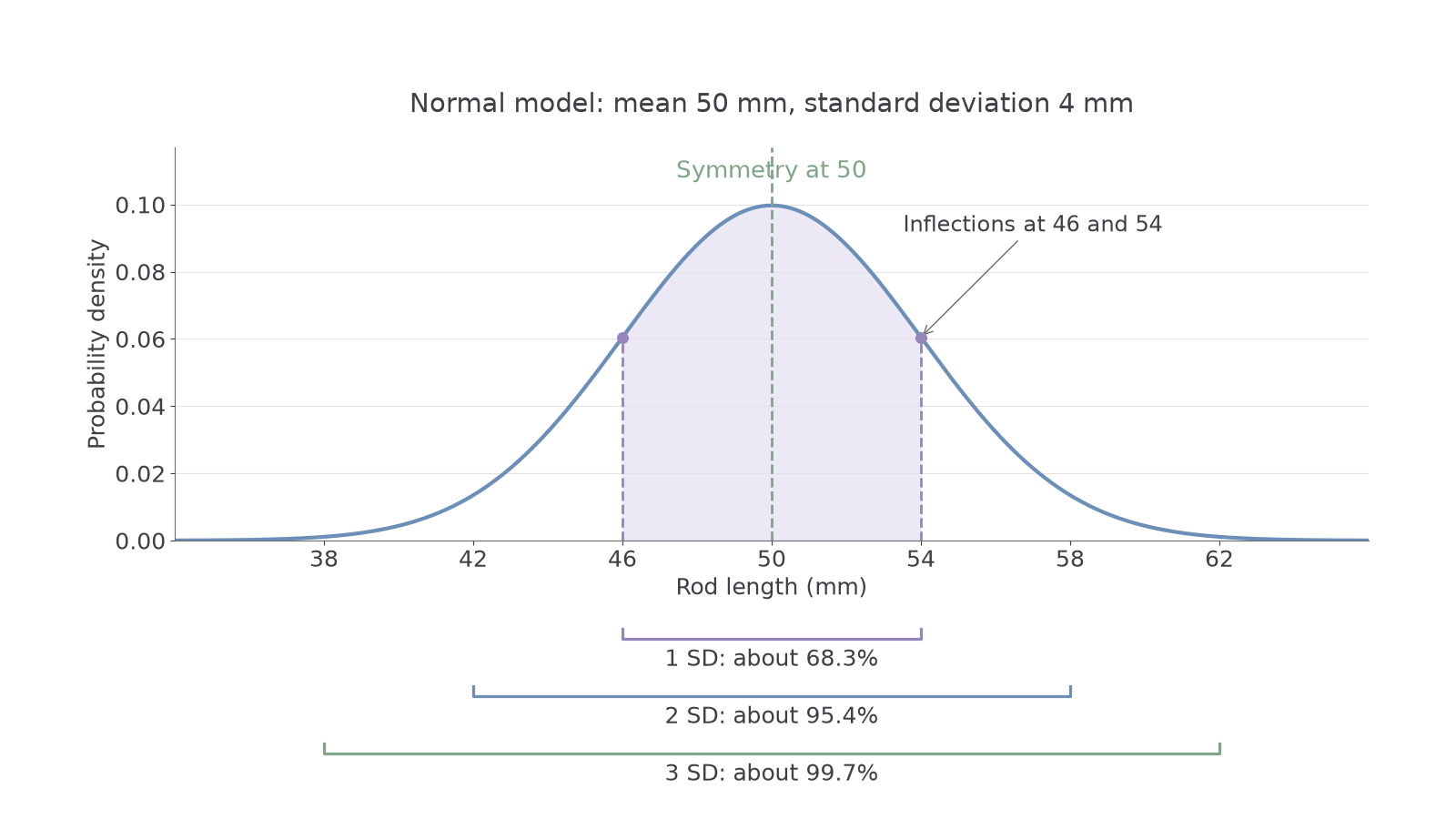
A surprisingly large majority fits within two standard deviations, but a normal model has no finite cut-off at three: the remaining tail probability is small, not zero.
Normal proportions and inflections
For a normal distribution,
Thus about two-thirds lie within one standard deviation, about 95% within two and almost all within three. Inflections occur at . These facts are not printed as such on the supplied sheet. Not in the formula sheet: learn it.
The corresponding rod-length intervals are 46–54, 42–58 and 38–62 mm. These proportions belong to the normal model; a different distribution need not follow them. Since an exact single value has zero probability in a continuous model, . This contrasts with the discrete spikes in the previous lesson.
Histograms from increasingly large samples of a normal population tend to reveal the normal shape more clearly, with suitable bins and random variation still present. Scale histogram area to 1 for comparison with the probability curve. Increasing widens the curve and lowers its peak, keeping total area 1; changing shifts it horizontally. You do not need the equation of the normal curve. A symmetric sample alone does not establish every tail prediction, and a normal model can assign tiny probabilities to physically impossible negative measurements; assess whether that matters in context.
Key idea
The mean locates the curve; the standard deviation sets distances along the measurement axis. Probability comes from area, never from reading a height.
Use the second parameter correctly before deciding which interval is appropriate.
Standardisation measures distance in standard deviations
Subtract the centre and divide by the spread to express a measurement's position on one common scale.
Standardising a normal variable
For ,
This is the standard normal distribution. Single-observation standardisation is not printed on the sheet; the sheet's expression for a sample mean uses a different standard deviation. Not in the formula sheet: learn it.
The result is unit-free, and the positive denominator preserves inequalities. Write . Symmetry gives ; in particular, . A calculator can also evaluate areas directly from the stated mean and standard deviation.
Worked example 1: a lower-tail area
Question. For rod lengths , find to three significant figures.
Plan. Standardise 56, then evaluate the area below that value.
Why this step? is already the area below the required cut-off; no complement is needed.
Answer. The probability is 0.933, to three significant figures.
Check. The upper tail is , answering the opening question. It is smaller than the roughly 16% above one standard deviation.
Change only the lower bound of the region: keep 56 as the upper cut-off but now start at 46 instead of extending indefinitely to the left.
Continue this lesson.
You’re previewing NovaLearn without an account. Create a free account to read the rest.
Create free account