1.02o, 1.02q - Reciprocal graphs, asymptotes and intersections | OCR A-Level Mathematics A

Use signs, excluded inputs and asymptotes to sketch reciprocal and inverse-square curves. You will solve their intersections exactly, then use supplied exponential and trigonometric graphs when algebra does not give a convenient answer.

The reciprocal curve

If you double an input, can its output halve while their product never changes? For $y=2/x$ , inputs 1, 2 and 4 give outputs 2, 1 and $\frac12$ . Every pair has product 2. The surprising part is that neither coordinate can ever be zero.

You already know

Division by zero is undefined. For nonzero numbers, a positive divided by a positive is positive; a positive divided by a negative is negative. Use these sign rules before plotting points.

The same fixed-product relationship works at negative inputs too: $(-1,-2)$ and $(-2,-1)$ also have product 2.

A reciprocal relationship

For fixed real $a\ne0$ ,

y=\frac ax\quad\Longleftrightarrow\quad xy=a,\qquad x\ne0.

If $a>0$ , the branches lie in quadrants I and III; if $a<0$ , they lie in quadrants II and IV. There are no axis intercepts. Replacing $x$ by $-x$ negates $y$ , giving symmetry about the origin.

Not in the formula sheet: learn it.

Plot each branch separately; there is no point at zero through which to join them.

Worked example 1: a positive reciprocal

Question. Describe the graph of $y=2/x$ , giving four points and any axis intercepts.

Plan. Calculate positive and negative input pairs and use the fixed nonzero product to rule out intercepts.

\begin{aligned} x=1,\ 2&\quad\Longrightarrow\quad y=2,\ 1 &&\text{positive inputs}\\ x=-1,\ -2&\quad\Longrightarrow\quad y=-2,\ -1 &&\text{negative inputs}\\ x=0&\quad\text{is excluded} &&\text{division by zero}\\ \frac2x=0&\quad\text{has no solution} &&\text{nonzero numerator} \end{aligned}

Why this step? Checking both input signs identifies both branches; a positive-only table would omit half the graph.

Answer. Smooth separate branches in quadrants I and III pass through $(1,2)$ , $(2,1)$ , $(-1,-2)$ , $(-2,-1)$ , with no intercepts.

Check. Each listed pair has product 2. Doubling 1 to 2 halves the output from 2 to 1.

Change only the numerator's sign. Every output reverses, but zero stays excluded.

Worked example 2: a negative reciprocal

Question. Describe the graph of $y=-2/x$ , giving the corresponding four points.

Plan. Negate the previous outputs and identify the resulting quadrants.

\begin{aligned} x=1,\ 2&\quad\Longrightarrow\quad y=-2,\ -1\\ x=-1,\ -2&\quad\Longrightarrow\quad y=2,\ 1\\ xy&=-2 &&\text{check the fixed product} \end{aligned}

Why this step? A negative numerator makes the input and output have opposite signs.

Answer. The branches are in quadrants II and IV, through $(1,-2)$ , $(2,-1)$ , $(-1,2)$ , $(-2,1)$ , with no intercepts.

Check. Each point has product $-2$ , and changing both coordinate signs leaves the relationship unchanged.

A model of this form is inverse proportion. Its physical domain may restrict it to positive inputs, even though the mathematical curve has two branches.

Watch out

Wrong: draw a segment through the origin joining the two branches.

Right: leave $x=0$ out completely. A reciprocal curve does not acquire a zero just because the axes cross there.

Change the numerator while keeping it negative.

Asymptotes describe limiting behaviour

An asymptote describes a line approached by a branch, rather than a missing point at a finite height.

For $y=2/x$ , inputs 10, 100 and 1000 give outputs $0.2$ , $0.02$ and $0.002$ . The outputs approach zero without equalling it. Inputs $0.1$ , $0.01$ and $0.001$ give 20, 200 and 2000, growing without bound as the input approaches zero.

Asymptote

An asymptote is a line approached by a curve in a specified limiting direction. For $y=a/x$ with $a\ne0$ , the horizontal asymptote is $y=0$ and the vertical asymptote is $x=0$ . These are equations of lines, not coordinates. The function has no value at zero; “infinity” is not its output there.

For these reciprocal curves, the numerator's sign and the side of zero tell you whether the unbounded values are positive or negative. The asymptote rules here are not in the formula sheet: learn them.

Worked example 3: approaching from both sides

Question. State the asymptotes of $y=2/x$ and describe its behaviour near zero and far from zero.

Plan. Evaluate inputs on both sides of zero and of large magnitude, then generalise their signs.

\begin{aligned} x=0.01&\quad\Longrightarrow\quad y=200 &&\text{near zero, positive side}\\ x=-0.01&\quad\Longrightarrow\quad y=-200 &&\text{near zero, negative side}\\ x=100&\quad\Longrightarrow\quad y=0.02\\ x=-100&\quad\Longrightarrow\quad y=-0.02 \end{aligned}

Why this step? “Approaches zero” for the input needs a side: the two branches become unbounded with opposite signs.

Answer. Asymptotes $x=0$ and $y=0$ . Near zero the right branch grows positively without bound and the left negatively without bound. Far to either side the outputs approach zero, with their respective signs.

Check. Multiplying each input by ten divides its output by ten, explaining both limiting patterns.

Change only the numerator's sign. The same lines are approached, but from opposite vertical directions.

Worked example 4: unchanged lines, reversed approach

Question. Describe the corresponding asymptotic behaviour of $y=-2/x$ .

Plan. Negate the four previous outputs, retaining the excluded input.

\begin{aligned} x=0.01&\quad\Longrightarrow\quad y=-200\\ x=-0.01&\quad\Longrightarrow\quad y=200\\ x=100&\quad\Longrightarrow\quad y=-0.02\\ x=-100&\quad\Longrightarrow\quad y=0.02 \end{aligned}

Why this step? Negating heights reverses the approach signs, but cannot move the lines $x=0$ and $y=0$ .

Answer. The asymptotes remain $x=0$ and $y=0$ . Near zero, the right branch is negatively unbounded and the left positively unbounded; far away, the outputs approach zero.

Check. A small positive denominator gives a large negative quotient, agreeing with the right branch in quadrant IV.

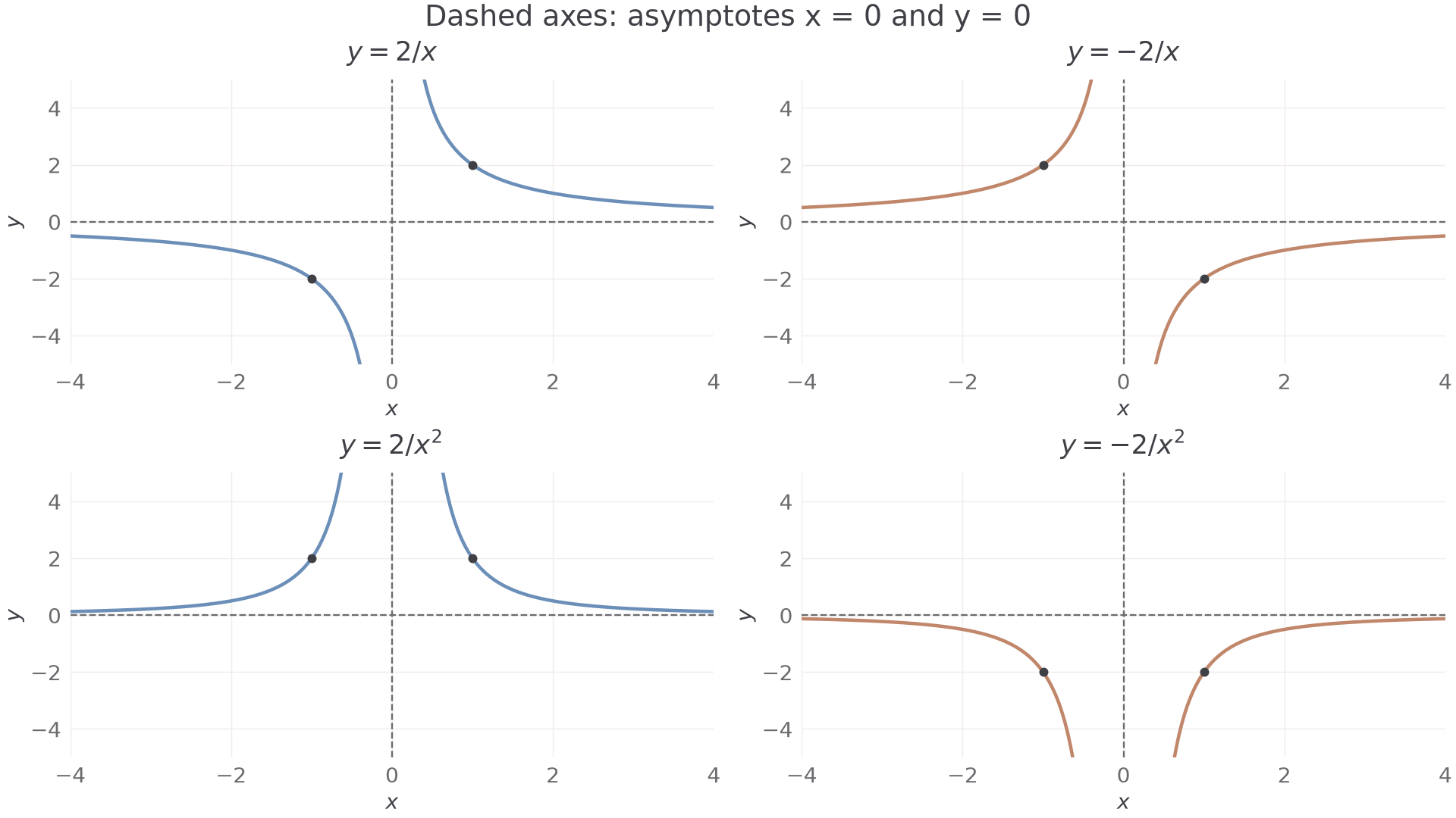
The top two panels show these reciprocal families. The lower two prepare the inverse-square comparison in the next part.

Positive and negative reciprocal and inverse-square families, with separate branches and asymptotic axes

An asymptote does not, in general, forbid a curve crossing that line elsewhere. These particular curves cannot cross $y=0$ because a nonzero numerator cannot give a zero quotient.

Watch out

Wrong: “At $x=0$ , $y=\infty$ .”

Right: the function is undefined at zero; its values grow without bound as permitted inputs approach zero from the stated side.

Apply the sign reasoning without needing a full table.

The inverse-square curve

Squaring the denominator changes the negative-input branch, because a nonzero square is always positive.

For $y=2/x^2$ , inputs 1 and $-1$ both give 2. Inputs 2 and $-2$ both give $\frac12$ . Opposite inputs now have equal outputs.

An inverse-square relationship

For fixed real $a\ne0$ ,

y=\frac a{x^2},\qquad x\ne0.

Both branches have the sign of $a$ , the graph is symmetric about the vertical axis, and its asymptotes are $x=0$ and $y=0$ . There are no axis intercepts. Doubling the input magnitude divides the output by four.

Not in the formula sheet: learn it.

Compare the lower panels of the diagram with the top panels: the sign change in the denominator is gone.

Worked example 5: positive on both sides

Question. Describe $y=2/x^2$ , including sample points, symmetry and behaviour near zero.

Plan. Square positive and negative inputs, then use the positive numerator.

\begin{aligned} x=\pm1&\quad\Longrightarrow\quad y=2 &&\text{denominator }1\\ x=\pm2&\quad\Longrightarrow\quad y=\frac12 &&\text{denominator }4\\ x=\pm0.1&\quad\Longrightarrow\quad y=200 &&\text{denominator }0.01 \end{aligned}

Why this step? Opposite inputs have the same square, explaining vertical-axis symmetry and equal signs on the two branches.

Answer. Both branches are above the horizontal axis, symmetric about the vertical axis. They grow positively without bound towards zero and approach $y=0$ as $|x|$ grows; $x=0$ is also an asymptote.

Check. Doubling the input magnitude from 1 to 2 changes the output from 2 to $\frac12$ , one quarter as large.

Change only the numerator to $-2$ . Both branches change sides together.

Worked example 6: negative on both sides

Question. Describe $y=-2/x^2$ in the same way.

Plan. Retain the squared denominator and negate every previous output.

\begin{aligned} x=\pm1&\quad\Longrightarrow\quad y=-2\\ x=\pm2&\quad\Longrightarrow\quad y=-\frac12\\ x=\pm0.1&\quad\Longrightarrow\quad y=-200 \end{aligned}

Why this step? It is the numerator, rather than the input sign, that determines the sign of an inverse-square output.

Answer. Both branches are below the axis, still symmetric about the vertical axis. They become negative without bound towards zero and approach $y=0$ far away; the vertical asymptote is $x=0$ .

Check. Inputs $-2$ and 2 give the same $-\frac12$ , so the left branch cannot lie above the axis.

The condition $a\ne0$ matters: if $a=0$ , the formula gives the horizontal line $y=0$ with zero excluded, rather than a vertical asymptote at zero.

Watch out

Wrong: $2/(-2)^2=-\frac12$ .

Right: square the whole negative input first: $2/(-2)^2=2/4=\frac12$ .

Distinguish reciprocal from inverse-square behaviour at a negative input.

Solve intersections without losing restrictions

To find an intersection, equate the heights and retain every restriction from the equations you started with.

You already know

At an intersection, both equations have the same $x$ and $y$ . Solving the resulting equation gives inputs; substitute each permitted input to recover its height.

Here $x=0$ is excluded before clearing any denominator. Multiplication cannot restore a point that never belonged to the curve.

Worked example 7: a reciprocal and a line

Question. Find all intersections of $y=6/x$ and $y=x+1$ .

Plan. Equate, multiply by the permitted nonzero input, factor and recover each height.

\begin{aligned} \frac6x&=x+1,\qquad x\ne0 &&\text{same height}\\ x^2+x-6&=0 &&\text{multiply by }x\\ (x+3)(x-2)&=0 &&\text{factor}\\ x&=-3,\ 2\\ y&=-2,\ 3 &&\text{substitute into the line} \end{aligned}

Why this step? Clearing the denominator is reversible on $x\ne0$ , so the resulting permitted roots can be checked in both equations.

Answer. $(-3,-2)$ and $(2,3)$ .

Check. $6/(-3)=-2=-3+1$ , and $6/2=3=2+1$ .

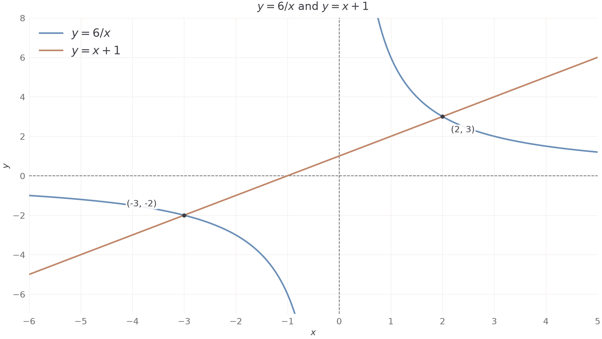
The exact points agree with the two visible crossings.

A reciprocal curve and line intersect at minus three, minus two and two, three

Change the comparison from a line to an inverse-square curve, keeping the first reciprocal curve fixed.

Worked example 8: two reciprocal families

Question. Find the intersection of $y=6/x$ and $y=3/x^2$ .

Plan. Equate outputs and multiply by $x^2$ , which is nonzero on the shared domain.

\begin{aligned} \frac6x&=\frac3{x^2},\qquad x\ne0\\ 6x&=3 &&\text{multiply by }x^2\\ x&=\frac12\\ y&=\frac6{1/2}=12 &&\text{recover the height} \end{aligned}

Why this step? Multiplying by the squared denominator removes both fractions in one step and keeps the nonzero restriction visible.

Answer. $\left(\frac12,12\right)$ is the only intersection.

Check. $3/(1/2)^2=3/(1/4)=12$ , matching the reciprocal output.

The equality and domain rules for intersections are not in the formula sheet: learn them. If exact algebra is unavailable, a complete scaled graph can instead supply approximate inputs and heights; the next part uses this with other curve families.

Watch out

Wrong: accept a denominator-zero input because it appears after rearranging.

Right: retain the starting domain throughout. A transformed equation may be defined at inputs where the starting curve is not.

Change the two numerators and use the same shared-domain method.

Intersections with supplied exponential and trigonometric graphs

The intersection principle works even when you cannot rearrange the equation into a familiar polynomial.

In the supplied graphs below, $2^x$ is an exponential curve: it has values $\frac12,1,2,4$ at inputs $-1,0,1,2$ . The second curve is $y=\sin x$ , the sine wave shown for angles measured in radians. You can use their displayed shapes and calculator values here without assuming later methods for solving exponential or trigonometric equations.

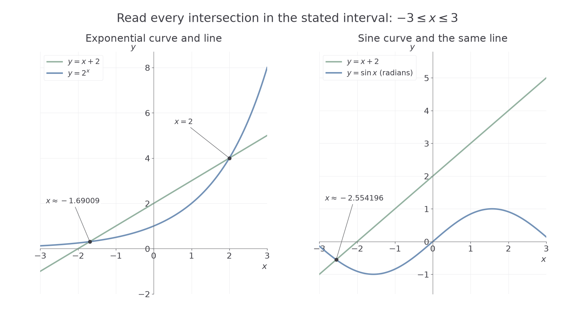
An exponential curve and a sine curve each compared with the same line on minus three to three

Read an intersection's horizontal coordinate as an approximate equation solution, then use either function for its height. This rule is not in the formula sheet: learn it.

Worked example 9: an exponential meeting a line twice

Question. Use the supplied exponential graph to solve $2^x=x+2$ for $-3\le x\le3$ , giving the solutions to 3 significant figures.

Plan. Read the two crossings of $y=2^x$ and $y=x+2$ , then use calculator substitution to check their approximate locations.

\begin{aligned} x&\approx-1.69009,\ 2 &&\text{intersection read-outs}\\ 2^{-1.69009}&\approx0.309908 &&\text{exponential height}\\ -1.69009+2&=0.309910 &&\text{line height}\\ 2^2&=4=2+2 &&\text{second crossing exact} \end{aligned}

Why this step? The graph identifies two roots in the specified interval; checking only the easy root 2 would miss the negative root.

Answer. $x\approx-1.69$ or $x=2$ .

Check. The near-equal heights at the negative input agree to the precision of the read-out. A graph reading alone would be approximate even when it happened to display an integer.

Change only the curve family in the comparison: the line remains $y=x+2$ , but it now meets the supplied sine wave.

Worked example 10: a trigonometric intersection

Question. Use the supplied sine graph to solve $\sin x=x+2$ for $-3\le x\le3$ , giving the solution to 3 significant figures.

Plan. Locate its single crossing with the same line, read the input and verify it in radian mode.

\begin{aligned} x&\approx-2.554196 &&\text{intersection read-out}\\ \sin(-2.554196)&\approx-0.554196 &&\text{radian evaluation}\\ -2.554196+2&=-0.554196 &&\text{line height} \end{aligned}

Why this step? Radians are part of the supplied graph's definition; degree-mode evaluation would compare a different curve with the line.

Answer. $x\approx-2.55$ is the only solution in the stated interval.

Check. The two calculated heights agree to 6 decimal places at the unrounded read-out. Use that unrounded input for checking rather than expecting rounded $-2.55$ to give exact equality.

A calculator's intersection tool reports a root in its chosen window, not automatically every root of the equation. Inspect the entire specified interval, including its endpoints. For the two examples the boundary inputs $-3$ and 3 are not roots.

Exam tip

State that graph readings are approximate and retain guard digits before rounding. H240's usual final accuracy is 3 significant figures unless the question specifies another accuracy; an exact solution needs algebra or another exact justification.

Change only the line's intercept in the sine comparison, and check a supplied intersection read-out.

Quick Recap

$a/x$ has a fixed nonzero coordinate product and opposite input signs give opposite output signs.
$a/x^2$ has equal outputs at opposite inputs; both branches have the numerator's sign.
Both families have asymptotes $x=0$ and $y=0$ , with zero excluded.
Equate heights for exact intersections; supplied graphs and calculator read-outs give approximate solutions for other curve families too.

Yes: doubling a reciprocal input halves its output while their product remains fixed. Zero can be neither input nor output when that fixed product is nonzero.

Last Accessed

Pure Mathematics

Statistics

Mechanics

1.02o, 1.02q - Reciprocal graphs, asymptotes and intersections

The reciprocal curve

Asymptotes describe limiting behaviour

The inverse-square curve

Solve intersections without losing restrictions

Intersections with supplied exponential and trigonometric graphs

Quick Recap

Learn faster with Nova