2.02a, 2.02b - Univariate diagrams, histograms and distributions | OCR A-Level Mathematics A

Read tables and single-variable diagrams in 2.02a, then use histogram area and evaluate display choices in 2.02b. You will learn why a taller bar can represent fewer people, and how to recover the information a graph actually contains.

Reading single-variable displays

Can a shorter histogram bar contain more people? In the 2011 census, County Durham had 28,574 residents aged 0–4 and 15,818 aged 5–7: those groups cover five years and three years, so their counts alone cannot tell us which age band has the taller density bar.

You already know

A proportion is a count divided by the relevant total. Read a graph's key, axis labels and units before using its numbers.

First distinguish the observations from their picture. A travel method is categorical, a journey count is discrete numerical, and a measured waiting time is continuous even if recorded to the nearest minute. A rank orders observations but does not measure equal gaps between them. Giving “walk” code 1 and “bus” code 2 does not make the average code a travel method.

Frequency

Frequency is the number of observations in a value, category or class. Relative frequency is its frequency divided by the total frequency. Grouping combines values into intervals and loses their individual positions.

The displays below use constructed small datasets so that every mark is readable.

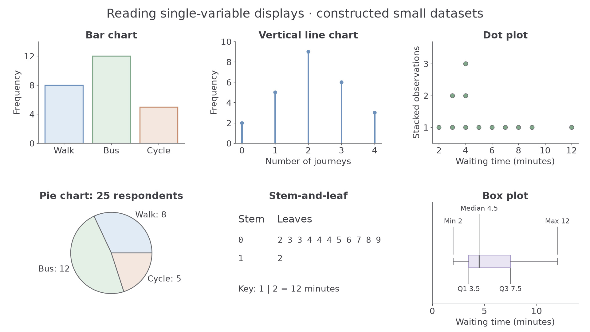
Ways to represent single-variable data

Display	Read this first	Useful information and limitation
Bar chart	Category labels and separated bar heights	Compares category counts; category order may be arbitrary.
Vertical line chart	Numerical positions and line heights	Keeps separate discrete values; a gap is not an unrecorded interval of continuous values.
Dot plot	Key and stacked dots	One dot per observation here; repeated values remain visible.
Stem-and-leaf	Key, every leaf and repeated leaves	Preserves actual values; becomes crowded for a large dataset.
Box plot	Median, quartiles and whisker definition	Summarises centre and spread; conceals detailed shape and sample size unless supplied.

A pie sector shows a proportion of a whole: 12 of 40 observations gives $(12/40)\times360^\circ=108^\circ$ . Non-standard displays need the same care: if one bicycle icon means eight commuters, five icons mean 40 commuters. If area represents count, twice the area means twice the count, not twice each side length.

Worked example 1: decoding a stem-and-leaf

Question. A display has key $2\mid4=24$ minutes and rows $1\mid6\;8\;8$ and $2\mid0\;3$ . Find the proportion of waits at least 20 minutes.

Plan. Decode each leaf, then count the observations meeting the threshold.

\begin{aligned} \text{times}&=16,18,18,20,23 &&\text{use the key}\\ \text{proportion}&=\frac{2}{5}=0.4 &&\text{two qualifying observations} \end{aligned}

Why count leaves? Each repeated leaf is another observation, so both 18s belong in the denominator.

Answer. The proportion is $0.4$ , or $40\%$ .

Check. Two qualifying leaves plus three other leaves gives five observations.

Change only the threshold in example 2. The dataset and its key stay fixed.

Worked example 2: a boundary that includes repeats

Question. For the same rows and key, find the proportion of waits at least 18 minutes.

Plan. Include equality at the threshold, including both repeated 18s.

\begin{aligned} \text{qualifying times}&=18,18,20,23 &&\text{at least includes equality}\\ \text{proportion}&=\frac{4}{5}=0.8 &&\text{divide by all five leaves} \end{aligned}

Why include both 18s? A threshold selects observations, not distinct numerical values.

Answer. $0.8$ , or $80\%$ .

Check. Only the 16-minute wait is below the threshold, giving $1-1/5=0.8$ .

A scale can also change the visual impression. Bars of 100 and 110 differ by $10\%$ relative to 100; an axis starting at 95 makes their visible heights 5 and 15, a misleading threefold visual ratio if the baseline is overlooked.

Watch out

Wrong: “The median is near the left edge of a box, so fewer observations are on that side.” Quartile sections represent approximately equal proportions, not equal lengths. Read labelled values rather than judging the amount of ink.

Try decoding a fresh set before comparing its proportions.

Histogram area represents frequency

A histogram shares frequency between both dimensions of a bar: its width and its height.

Histogram

A histogram represents grouped numerical data using touching bars whose areas are proportional to class frequencies. With a frequency-density axis, each bar's area equals its frequency numerically.

The width is the difference between class boundaries. For ages in completed years, ages 0–4 cover the continuous age interval from birth up to age 5, a width of five years; ages 5–7 cover ages 5 to under 8, a width of three years.

Frequency density

For a class of positive width:

\text{density}=\frac{\text{frequency}}{\text{width}},\qquad \text{frequency}=\text{width}\times\text{density}.

Dividing a class frequency by the total gives its relative frequency, estimating the probability of that class under an appropriate sampling model.

Not in the formula sheet: learn it.

Consider this constructed table of 50 waits. The diagram shows why a bar's height alone is insufficient.

Time $t$ , minutes	Frequency	Width	Density
$0\le t<5$	10	5	2
$5\le t<10$	20	5	4
$10\le t<20$	15	10	1.5
$20\le t\le30$	5	10	0.5

Histogram and cumulative frequency for 50 waits

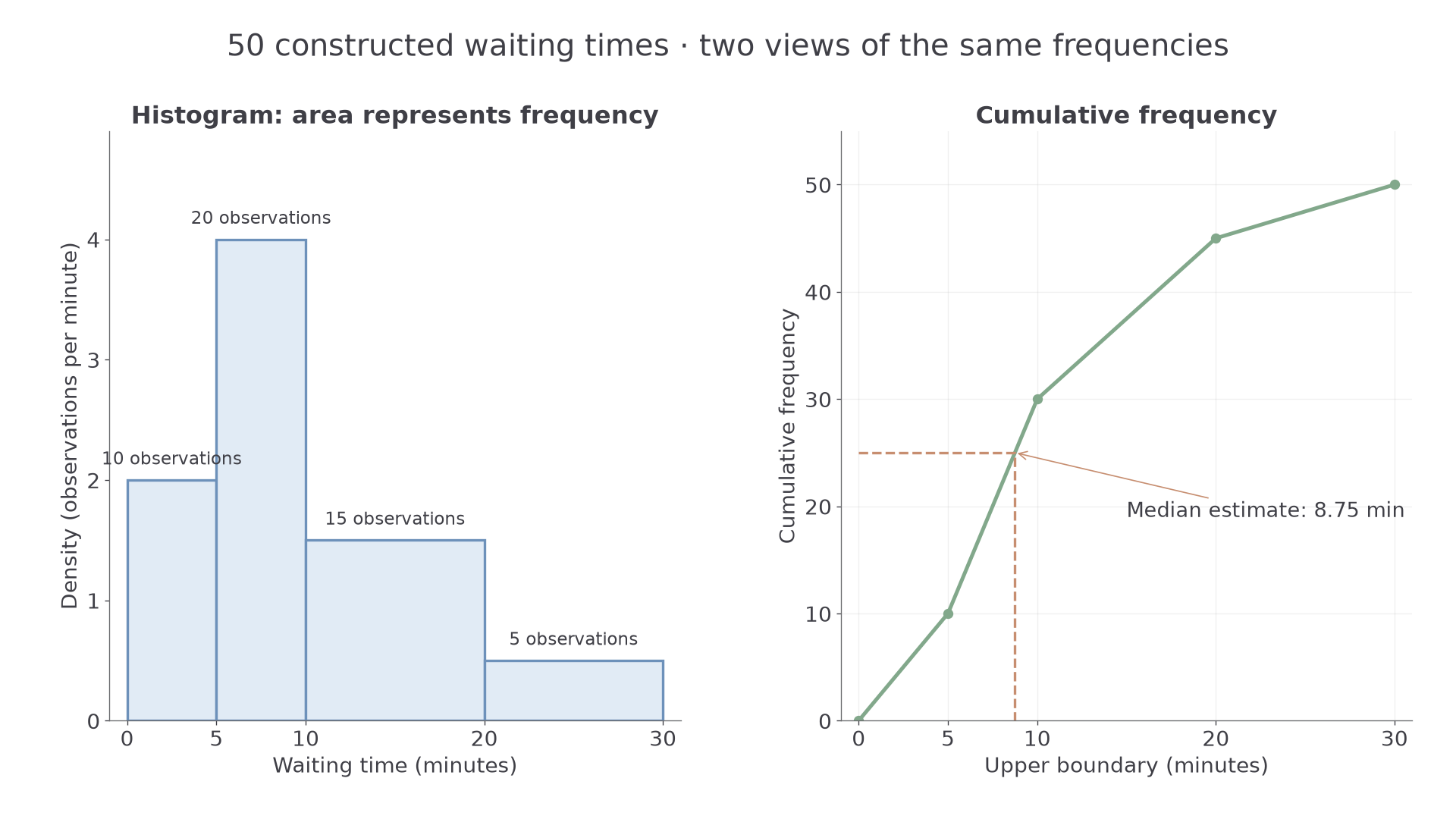
The total area is 50. The 10–20-minute class therefore represents proportion $15/50=0.30$ . Dividing all heights by 50 would give a relative-frequency-density histogram with total area 1, a bridge to continuous probability distributions.

Worked example 3: finding a density

Question. Twenty observations occupy the class $5\le x<10$ . Find its frequency density.

Plan. Divide the frequency by the width between the boundaries.

\begin{aligned} w&=10-5=5 &&\text{class width}\\ d&=\frac{20}{5}=4 &&\text{frequency per unit width} \end{aligned}

Why divide? The height must spread 20 observations over five horizontal units.

Answer. Frequency density $4$ .

Check. $5\times4=20$ , recovering the bar's frequency.

Change only the upper class boundary; keep the same 20 observations.

Worked example 4: the same frequency in a wider class

Question. Twenty observations occupy $5\le x<15$ . Find the frequency density.

Plan. Recalculate the width before dividing the unchanged frequency.

\begin{aligned} w&=15-5=10 &&\text{new width}\\ d&=\frac{20}{10}=2 &&\text{same frequency spread further} \end{aligned}

Why does the height halve? Doubling the width must halve the height to preserve area.

Answer. Frequency density $2$ .

Check. $10\times2=20$ , the same area as before.

Continue this lesson.

You’re previewing NovaLearn without an account. Create a free account to read the rest.

Create free account

Last Accessed

Pure Mathematics

Statistics

Mechanics

2.02a, 2.02b - Univariate diagrams, histograms and distributions

Reading single-variable displays

Histogram area represents frequency

Continue this lesson.

Learn faster with Nova