1.02m, 1.02n, 1.02p - Polynomial graphs, roots and intercepts | OCR A-Level Mathematics A

Connect a polynomial's factors to its intercepts, crossings and end behaviour. You will turn those clues into a sketch, use stationary-point information when needed and interpret algebraic solutions as graph intersections.

Plotting and sketching a graph

Can a cubic meet the horizontal axis twice but cross it only once? The curve $y=(x+2)(x-1)^2$ does exactly that. We will explain the apparent puzzle using factors, then locate the turning points that complete its shape.

Start with a simpler curve. For $y=x^2-1$ , inputs $-2,-1,0,1,2$ give outputs $3,0,-1,0,3$ . These points belong to a smooth parabola, rather than a chain of straight segments.

Plot and sketch

To plot a graph, calculate and mark accurate points on scaled axes. To sketch a graph, show its principal features and their relationships: labelled axes, intercepts, shape, end directions and any required turning points. A sketch need not be to scale, but exact known coordinates must be labelled correctly.

A short point table can miss a feature between its inputs. Algebra tells you which features must be there.

You already know

The square in $y=a(x-h)^2+k$ is zero at $x=h$ . If $a>0$ , the minimum is $(h,k)$ ; if $a<0$ , this is a maximum. Set $y=0$ for horizontal intercepts and $x=0$ for the vertical intercept.

Use the completed-square form to build a sketch without a long table.

Worked example 1: sketching from a square

Question. State the features needed to sketch $y=(x-1)^2-4$ .

Plan. Read the minimum, solve for the horizontal intercepts and substitute zero for the vertical intercept.

\begin{aligned} (x-1)^2&\ge0 &&\text{non-negative square}\\ y_{\min}&=-4\quad\text{at }x=1 &&\text{square is zero}\\ 0=(x-1)^2-4&\quad\Longrightarrow\quad x-1=\pm2 &&\text{horizontal intercepts}\\ x&=-1,\ 3\\ y(0)&=1-4=-3 &&\text{vertical intercept} \end{aligned}

Why this step? The completed square gives the minimum immediately; expanding first would hide that information.

Answer. Draw an upward parabola with minimum $(1,-4)$ , crossings $(-1,0)$ and $(3,0)$ , and vertical intercept $(0,-3)$ . Its symmetry line is $x=1$ .

Check. The two roots lie equally far from 1, and substituting either gives zero.

Change only the overall sign of the function. This reverses every height, including the minimum's height.

Worked example 2: reversing the heights

Question. State the features needed to sketch $y=-(x-1)^2+4$ .

Plan. Read the maximum and check which intercepts change when every output is negated.

\begin{aligned} -(x-1)^2&\le0 &&\text{negative square}\\ y_{\max}&=4\quad\text{at }x=1\\ 0=-(x-1)^2+4&\quad\Longrightarrow\quad(x-1)^2=4 &&\text{same zero heights}\\ x&=-1,\ 3\\ y(0)&=-1+4=3 &&\text{vertical intercept reverses} \end{aligned}

Why this step? Negating zero still gives zero, so the horizontal intercepts stay fixed while the other heights reverse.

Answer. Draw a downward parabola with maximum $(1,4)$ , crossings $(-1,0)$ , $(3,0)$ , and vertical intercept $(0,3)$ .

Check. At $x=1$ , the output is 4; at $x=0$ and 2, it is 3 on both sides of the symmetry line.

The vertex and intercept rules used here are not printed in the formula sheet: learn them. A sketch is a statement about the whole shape, not a guess through one calculated point.

Watch out

Wrong: join a few polynomial points with straight segments.

Right: use a smooth curve with the correct features. A sharp corner would assert behaviour that this polynomial does not have.

Change the centre and depth of the first parabola in your own sketch description.

Factors reveal roots and crossings

The factors tell you both where a polynomial meets the axis and whether its sign changes there.

Root and multiplicity

A real root of $\mathrm f(x)=0$ is an input $r$ with $\mathrm f(r)=0$ ; the corresponding intercept is the point $(r,0)$ . Its multiplicity is the number of copies of the factor $(x-r)$ . For example, $(x-1)^2$ gives multiplicity two at 1, not a root at $-1$ .

Close to a root, all the other nonzero factors keep their signs. The factor that vanishes decides whether the product changes sign.

Crossing or touching

If $\mathrm f(x)=(x-r)^m\mathrm g(x)$ , where $m$ is a positive integer and $\mathrm g(r)\ne0$ , the graph crosses the axis at $r$ for odd $m$ and touches without crossing for even $m$ .

Not in the formula sheet: learn it.

A square stays positive on either side of its zero. An odd power changes sign.

Worked example 3: a repeated root that touches

Question. Find the intercepts and crossing behaviour of $\mathrm f(x)=(x+2)(x-1)^2$ .

Plan. Set each factor to zero, count its multiplicity and evaluate $\mathrm f(0)$ .

\begin{aligned} x+2=0&\quad\Longrightarrow\quad x=-2 &&\text{multiplicity one}\\ (x-1)^2=0&\quad\Longrightarrow\quad x=1 &&\text{multiplicity two}\\ \mathrm f(0)&=2(-1)^2=2 &&\text{vertical intercept} \end{aligned}

Why this step? The square has the same positive sign on both sides of 1, so this root cannot change the product's sign.

Answer. The curve crosses at $(-2,0)$ , touches at $(1,0)$ , and passes through $(0,2)$ .

Check. Near 1, the factor $x+2$ is positive and the square is positive on both sides, so the curve stays above the axis.

Change only the repeated factor's power, from two to three. A repeated root can now cross.

Worked example 4: a repeated root that crosses

Question. Find the intercepts and crossing behaviour of $\mathrm g(x)=(x+2)(x-1)^3$ .

Plan. Keep the same root positions but use the new odd multiplicity at 1.

\begin{aligned} x&=-2\quad\text{with multiplicity 1} &&\text{first factor}\\ x&=1\quad\text{with multiplicity 3} &&\text{cubed factor}\\ \mathrm g(0)&=2(-1)^3=-2 &&\text{vertical intercept} \end{aligned}

Why this step? Cubing preserves a signed input's sign, so $(x-1)^3$ changes from negative to positive at 1.

Answer. The graph crosses at both $(-2,0)$ and $(1,0)$ , with a flattened crossing at 1, and passes through $(0,-2)$ .

Check. At $x=\frac12$ , the product is $-\frac5{16}$ ; at $x=\frac32$ , it is $\frac7{16}$ . The sign changes across 1.

The picture contrasts a cubic with one touch and a quartic with two touches.

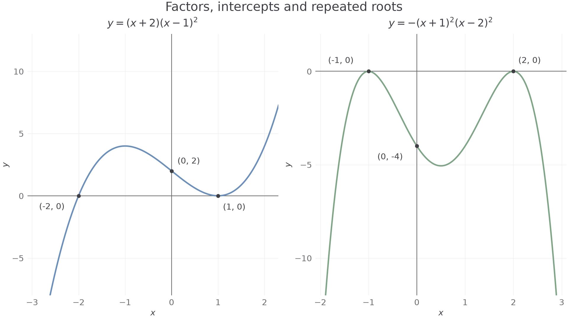
A cubic crosses at minus two and touches at one; a negative quartic touches at minus one and two

In the right panel, both zero-producing factors are squared, so both roots are touches.

Watch out

Wrong: every repeated root is a touch.

Right: even multiplicity gives a touch; odd multiplicity gives a crossing. The number of copies matters, not merely whether a factor repeats.

Use the same odd-multiplicity reasoning with two new roots.

Degree and sign determine the ends

The leading term controls the distant ends of a polynomial graph, while its factors control what happens at its roots.

For a concrete comparison, $x^3$ becomes negative far to the left and positive far to the right. In $x^3-3x+2$ , the cubic term eventually dominates the linear term and constant, so the same end directions apply.

Polynomial end behaviour

For a polynomial with leading term $ax^n$ , where $a\ne0$ and $n$ is a positive integer, the ends behave like $ax^n$ .

Degree	$a>0$	$a<0$
Even	Both ends up	Both ends down
Odd	Left down, right up	Left up, right down

Not in the formula sheet: learn it.

A sketch combines these end directions with every intercept and the sign between roots. End behaviour alone cannot locate every turn.

Worked example 5: assembling a cubic

Question. Describe a sketch of $\mathrm f(x)=(x+2)(x-1)^2$ .

Plan. Combine its leading term, intercepts and signs; leave any uncalculated turning height unlabelled.

\begin{aligned} \mathrm f(x)&=x^3-3x+2 &&\text{expand to identify leading term}\\ \mathrm f(0)&=2 &&\text{vertical intercept}\\ \mathrm f(x)&<0\quad(x<-2) &&\text{square positive, first factor negative}\\ \mathrm f(x)&>0\quad(-2<x<1\ \text{or}\ x>1) &&\text{both factors positive} \end{aligned}

Why this step? The sign intervals prevent an extra crossing being drawn between the stated roots.

Answer. Start down on the left, cross at $(-2,0)$ , pass through $(0,2)$ , touch at $(1,0)$ , then rise to the right. A turn above the axis is needed before the touch; the next part finds it exactly.

Check. The leading term is $x^3$ , agreeing with opposite end directions.

Change only the overall coefficient's sign and magnitude. The roots stay put, while every height is multiplied by $-2$ .

Worked example 6: a negative leading coefficient

Question. Describe the key sketch features of $\mathrm p(x)=-2(x+2)(x-1)^2$ .

Plan. Retain the root multiplicities and reverse the height signs and end directions.

\begin{aligned} \mathrm p(x)&=-2x^3+6x-4 &&\text{leading term }-2x^3\\ \mathrm p(0)&=-4 &&\text{vertical intercept}\\ \mathrm p(x)&>0\quad(x<-2) &&\text{sign reversed}\\ \mathrm p(x)&<0\quad(-2<x<1\ \text{or}\ x>1) \end{aligned}

Why this step? A nonzero overall coefficient changes no roots or multiplicities, but a negative one reverses all nonzero outputs.

Answer. Left end up, right end down; cross at $(-2,0)$ , touch at $(1,0)$ , and pass through $(0,-4)$ .

Check. At $x=-3$ , the output is 32, while at $x=2$ it is $-8$ , matching the end signs.

The quartic in the diagram has leading term $-x^4$ , so both ends go down. Since $-(x+1)^2(x-2)^2\le0$ , it touches at $-1$ and 2 and has vertical intercept $(0,-4)$ . Even degree does not guarantee real roots: $x^4+1\ge1$ never meets the horizontal axis.

Watch out

Wrong: “It is degree four, so it has four real crossings.”

Right: degree controls end behaviour and bounds the number of roots. Real roots may repeat, and some polynomial graphs have no real roots at all.

Keep the negative cubic coefficient, but move one root in the next check.

Locating and classifying stationary points

A stationary point has a horizontal tangent, and its position can complete a sketch that roots alone leave unfinished.

The tangent gradient is the local slope of a smooth curve. Write its gradient function as $\mathrm f'(x)$ : positive means rising from left to right, negative means falling, and zero means a horizontal tangent. You do not need a later differentiation method to use a supplied gradient function here.

Stationary point

A stationary point is a point where $\mathrm f'(x)=0$ . A change from positive to negative gradient gives a local maximum; negative to positive gives a local minimum. If the gradient does not change sign, a stationary point need not be a turning point: $y=x^3$ has a horizontal tangent at zero but rises on both sides.

For the opening cubic, the gradient function is $\mathrm f'(x)=3x^2-3$ . This is the slope of $x^3-3x+2$ at each input; it is supplied for the examples below. Stationary-point and gradient-sign rules are not in the formula sheet: learn them.

Worked example 7: the missing turn of the opening cubic

Question. Find and classify the stationary points of $\mathrm f(x)=x^3-3x+2$ , given $\mathrm f'(x)=3x^2-3$ .

Plan. Set the gradient to zero, substitute into the curve and inspect the gradient signs on either side.

\begin{aligned} 3x^2-3=0&\quad\Longrightarrow\quad x=-1,\ 1 &&\text{horizontal tangents}\\ \mathrm f(-1)&=-1+3+2=4 &&\text{curve height}\\ \mathrm f(1)&=1-3+2=0 &&\text{curve height} \end{aligned}

The gradient $3(x-1)(x+1)$ has signs positive, negative, positive across the intervals separated by $-1$ and 1.

Why this step? Zero gradient locates candidates; the change of sign distinguishes a maximum from a minimum.

Answer. Local maximum $(-1,4)$ and local minimum $(1,0)$ . Add these labels to the earlier sketch.

Check. At inputs $-2,0,2$ , the gradient values are $9,-3,9$ , confirming rise, fall, rise.

Now negate the whole cubic. The stationary inputs stay the same, but their classifications reverse.

Worked example 8: reversing the stationary features

Question. Find and classify the stationary points of $\mathrm h(x)=-x^3+3x-2$ , given $\mathrm h'(x)=-3x^2+3$ .

Plan. Solve the zero-gradient equation and use the new gradient signs.

\begin{aligned} -3x^2+3=0&\quad\Longrightarrow\quad x=-1,\ 1 &&\text{stationary inputs}\\ \mathrm h(-1)&=1-3-2=-4\\ \mathrm h(1)&=-1+3-2=0 \end{aligned}

The gradient signs are now negative, positive, negative.

Why this step? Negating all heights also negates every slope: a rise becomes a fall and a fall becomes a rise.

Answer. Local minimum $(-1,-4)$ and local maximum $(1,0)$ .

Check. The supplied gradient gives $-9,3,-9$ at $-2,0,2$ , matching those classifications.

The two complete sketches make the reversal visible.

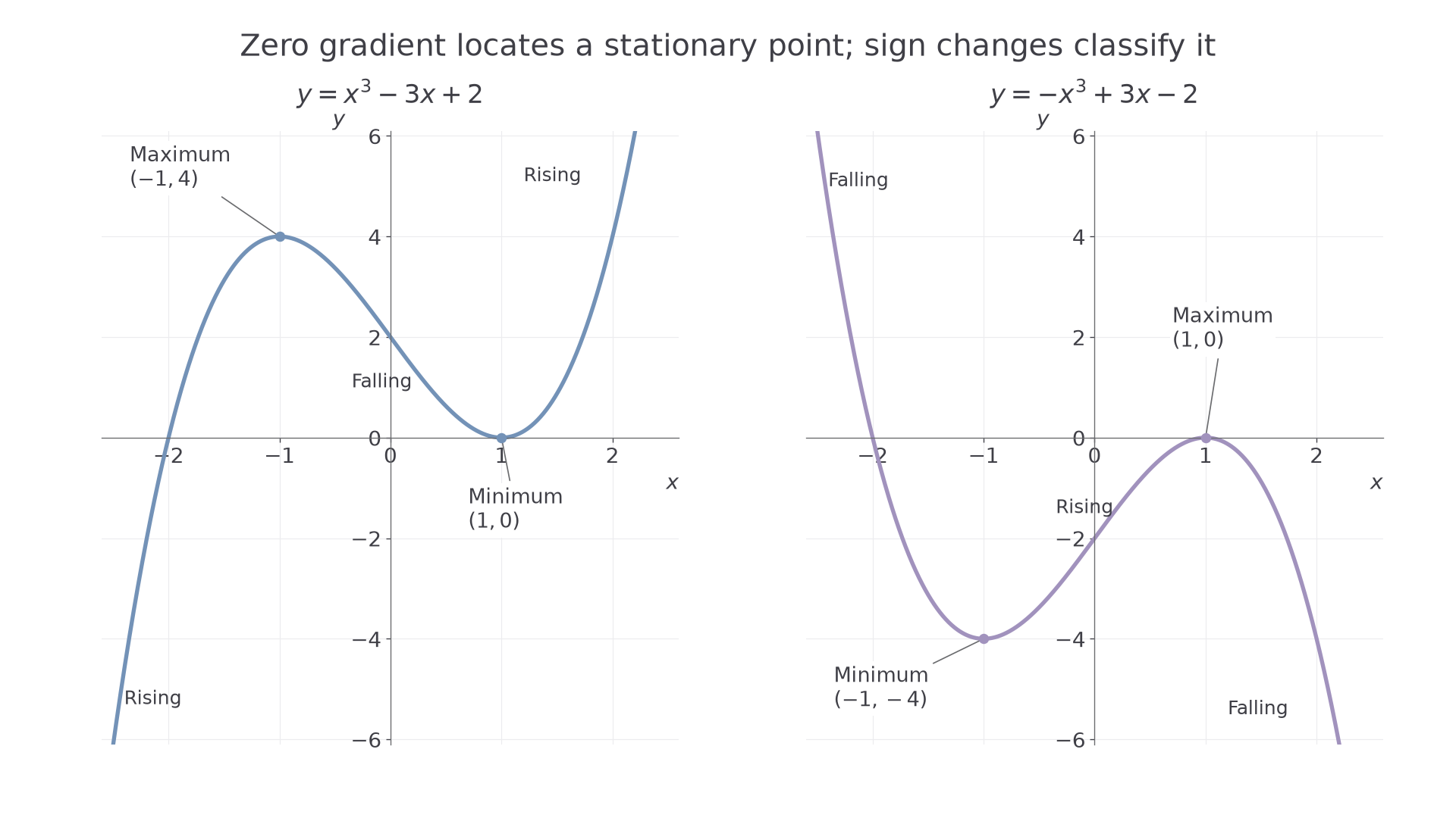
A cubic and its negative with every stationary point labelled and rising and falling intervals indicated

Use the curve equation for heights; the gradient equation gives slopes, not heights.

Watch out

Wrong: $\mathrm f'(1)=0$ , so every stationary point has coordinates $(1,0)$ .

Right: the second coordinate is $\mathrm f(1)$ . Zero is the gradient, not necessarily the height.

Apply the same supplied-gradient method with stationary inputs further apart.

Equation solutions are intersections

An algebraic equation has a graphical meaning: its solutions are the horizontal coordinates where the corresponding graphs meet.

For $\mathrm f(x)=0$ , the second graph is the horizontal axis. For $\mathrm f(x)=c$ , it is the line $y=c$ . For two simultaneous equations, recover the common vertical coordinate as well.

Intersections and simultaneous solutions

At an intersection of $y=\mathrm f(x)$ and $y=\mathrm g(x)$ ,

\mathrm f(x)=\mathrm g(x).

Each admissible solution $r$ gives the point $(r,\mathrm f(r))$ . An equation solution is an input; a simultaneous solution is an ordered pair.

Not in the formula sheet: learn it.

The graph helps you see the answer count, while algebra makes the coordinates exact.

Worked example 9: interpreting two algebraic roots

Question. Find the intersections of $y=x^2$ and $y=x+2$ , and interpret the roots of their intersection equation.

Plan. Equate heights, factor the resulting quadratic and substitute each root into the line.

\begin{aligned} x^2&=x+2 &&\text{equal heights}\\ (x-2)(x+1)&=0 &&\text{collect and factor}\\ x&=-1,\ 2\\ y&=1,\ 4 &&\text{substitute into }y=x+2 \end{aligned}

Why this step? Each root gives only a horizontal coordinate. Its matching height is needed for a point of intersection.

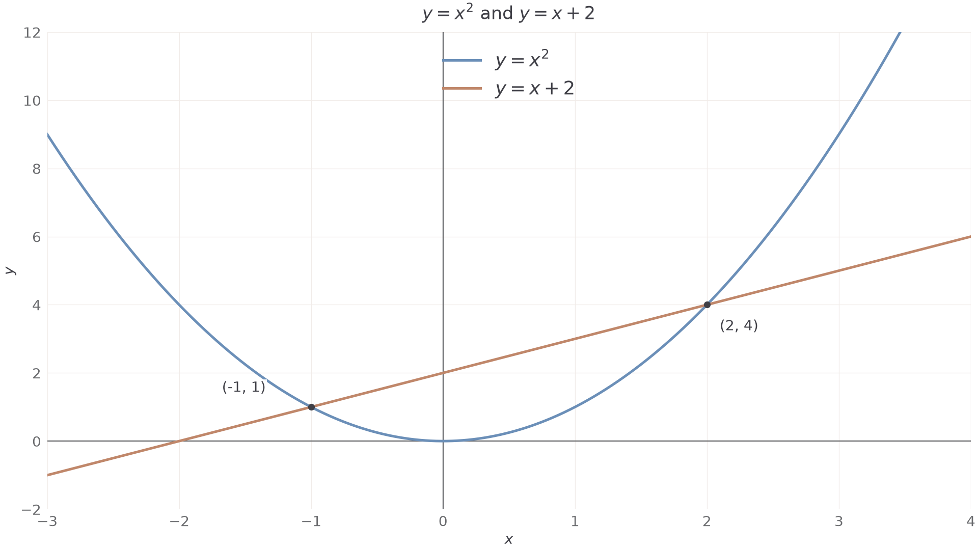
Answer. The intersections are $(-1,1)$ and $(2,4)$ . The solutions of $x^2=x+2$ are $-1$ and 2.

Check. Both pairs satisfy both equations: $(-1)^2=1=-1+2$ and $2^2=4=2+2$ .

The two crossings below correspond exactly to the two factors above.

The parabola y equals x squared and line y equals x plus two meeting at minus one, one and two, four

Change only the line's intercept so that $y=x$ replaces $y=x+2$ .

Worked example 10: a changed line intercept

Question. Find the intersections of $y=x^2$ and $y=x$ .

Plan. Equate the two outputs, factor out $x$ , then find both heights.

\begin{aligned} x^2-x&=0 &&\text{equate and collect}\\ x(x-1)&=0 &&\text{factor, do not divide by }x\\ x&=0,\ 1\\ y&=0,\ 1 &&\text{substitute into the line} \end{aligned}

Why this step? Factoring retains the solution $x=0$ , which dividing by $x$ would lose.

Answer. $(0,0)$ and $(1,1)$ .

Check. Each point gives the same value for $x^2$ and $x$ .

A tangent can give one repeated intersection root; a line missing a parabola gives no real roots. Read exact values from algebra, rather than assigning false precision to a sketch.

Exam tip

For “Find the points of intersection”, give ordered pairs. A list of roots answers only the horizontal-coordinate part of the problem.

Move the line again and recover every requested coordinate.

Quick Recap

A sketch shows principal features; a plot uses accurate points and scales.
A root of odd multiplicity crosses the axis; a root of even multiplicity touches it.
The leading term controls the distant ends, while gradient signs classify stationary points.
Algebraic roots are intersection inputs; simultaneous solutions include their common heights.

The opening cubic meets the axis at $-2$ and 1 but crosses only at $-2$ : the root at 1 is doubled. Its stationary points are $(-1,4)$ and $(1,0)$ .

Last Accessed

Pure Mathematics

Statistics

Mechanics

1.02m, 1.02n, 1.02p - Polynomial graphs, roots and intercepts

Plotting and sketching a graph

Factors reveal roots and crossings

Degree and sign determine the ends

Locating and classifying stationary points

Equation solutions are intersections

Quick Recap

Learn faster with Nova