2b, 2c - Exploring the 2027 large data set
Turn the prescribed census workbook into questions you can investigate, rather than a wall of numbers. You will use its metadata, spreadsheet calculations, graphs and repeated samples to make defensible claims, then connect those habits to graphing and algebra software across mathematics.
The workbook describes authorities in two censuses
How can Gateshead's bus-travel share fall from about to , while its number of bus travellers rises from to ? A percentage has a denominator as well as a numerator. This real census comparison will keep us honest throughout the lesson.
You already know
A percentage is times a proportion. A sample describes selected members of a population; the population and the unit selected must be named before a statistic has a clear meaning.
The prescribed H240 large data set contains travel-to-work and age-structure tables for aligned local authority areas in England and Wales, in the and censuses. It is the fixed H240 resource used for , rather than MEI's changing sequence of data sets. Open the census workbook, student notes and source information. The census data are from ONS, under Open Government Licence v3.0.
Observational unit
The observational unit is the entity described by one data row. Here a row describes one local authority area, not one resident or one journey. A count within that row can describe many residents.
Read the Information sheet before choosing columns. In a travel table, the method is the one used for the longest part by distance of the usual journey to work, among people in employment in the week before the census. Someone recorded as using a train might also walk or drive for another stage. Use the employment count for a travel proportion. The age tables instead count usual residents; age is age at the last birthday, age bands contain counts, and mean and median age have units of years.
The mean of authority percentages gives each authority equal weight. Dividing total bus travellers by total employment weights authorities by their employment counts. These are different questions; neither calculation repairs a badly chosen denominator.
Key idea
Before calculating, finish the sentence: “One row is …, my variable is …, and my denominator counts …”. Familiarity with the context matters; memorising hundreds of values does not. The full workbook is unavailable in the examination, where selected data or summaries may be supplied.
Try applying that sentence to a travel-method claim.
Metadata sets the limits of a comparison
Matching names is a risky way to join two census tables; matching their nine-character geography codes identifies the aligned areas directly.
The first three characters tell you the type of area. They are useful context, not a numerical measurement to average.
| Prefix | Area type |
|---|---|
| E06 | Unitary authority in England |
| E07 | Non-metropolitan district in England |
| E08 | Metropolitan borough in England |
| E09 | London borough |
| W06 | Unitary authority in Wales |
For example, County Durham's code E06000047 belongs to the first family. Some unitary authorities were formed by combining districts in ; the workbook adds their counts to match the later areas. County Durham combines seven former districts. You can compare the combined area across the two dates, but cannot recover those seven separate district results from their sum. That is lost geographical detail, not a spreadsheet error.
Metadata and imputation
Metadata explains what data mean and how they were obtained or organised. Imputation replaces an invalid or unavailable response using an estimation procedure. It does not mean that the replacement was directly observed.
The age metadata matters too. In , dates of birth implying ages above were treated as invalid and age was imputed; in , the cut-off was . An infant below one year is recorded as age . The open-ended “Age 90 and over” group therefore has different effective upper limits across the two censuses. A midpoint estimate must state its choice; a change in an estimate may reflect that convention as well as population change.
Mean and median age were not retained in the workbook. Grouped age counts cannot reveal exact individual ages, so they cannot reconstruct the exact mean or median. If exact means and population counts of all constituent districts were available, their population-weighted mean would recover the combined mean. Averaging district medians would still not recover the combined median: the combined middle position depends on the individual age distributions. Published rounded means would only give an approximate combined mean.
Watch out
Wrong: treat every W06 area as having the same population or transport pattern because its prefix agrees. Right: the prefix identifies an administrative type. Size, settlement and travel patterns still vary between Welsh authorities.
A comparison needs common definitions as well as matching areas.
Filtering and formulas need explicit denominators
A spreadsheet calculation becomes reproducible when another person can identify your columns, cleaning choices, selected rows and denominator.
Keep the source unchanged and make a working copy. On “Method of Travel by LA 2011”, select geography code, Region, authority name, employment and bus/minibus/coach. Copy these to columns A–E of a new sheet, with headers in row , and put bus percent in F. For data row , enter , then fill down. A cell is a column-and-row address, such as D2; filling down should change the row references, so the next formula uses E3 and D3.
Locate fields by header, not remembered position. Taxi is column L in , but I in . In the supplied travel sheet P is blank and Q contains people not in employment; exclude that separate count from employment denominators. The Isles of Scilly underground cell contains a dash. OCR's official notes recommend replacing this dash by zero in a working copy; record that documented cleaning decision. Do not generalise “dash means zero” to other data sets. Missing mean and median ages remain unavailable.
Travel percentage
For an authority with positive employment count and recorded bus count ,
Here is a percentage, not a fraction. The employment denominator must refer to the same area and census as the numerator. Not in the formula sheet: learn it.
Filtering Region to North East selects authorities. The first two give a quick check on the filled formula.
Worked example 1: the first selected authority
Question. County Durham has employed residents and recorded bus travellers in . Calculate the bus percentage to significant figures.
Plan. Divide the travel count by the matching employment count, then convert the fraction to a percentage.
Why this step? The travel categories describe employed residents, so using the larger age-table population would answer a different question.
Answer. County Durham's bus percentage was .
Check. of is about , close to the recorded count.
Change only the authority in Worked example 2. The census, variable, denominator rule and precision stay the same.
Worked example 2: the next selected authority
Question. Darlington has employed residents and recorded bus travellers in . Calculate the bus percentage to significant figures.
Plan. Apply the same percentage calculation to Darlington's own row.
Why this step? Copying a numerator from one row and a denominator from another would create a percentage belonging to neither authority.
Answer. Darlington's bus percentage was .
Check. It is a little below , since , slightly above .
For the whole North East, copy the selected complete rows to a compact analysis range. Ordinary and still include hidden rows; a filter alone is not a safe range definition. In F2:F13, checks the count, gives , and gives percentage points. Here all selected authorities are the defined group, so the SD uses divisor , consistent with H240's formula sheet.
The pooled percentage is instead
The mean of the percentages is ; the pooled percentage is . Unequal employment counts explain the difference.
Watch out
Wrong: replace every non-number by zero before calculating. Right: read what the code means. A documented zero travel count can be converted to zero; unavailable age summaries cannot.
Now change the authority once more, then check that the spreadsheet has selected the intended group.
Graphs turn a question into inspectable evidence
State a question before choosing a graph: “Did the bus percentage fall between the two censuses in North East authorities?” calls for matched comparisons, not one pooled bar.
Join the two travel tables by geography code, keeping each year's employment denominator with its bus count. Select authority labels and the two computed percentage columns. A grouped bar chart puts both years beside each other on one percentage scale; the graph below uses all matched North East areas.
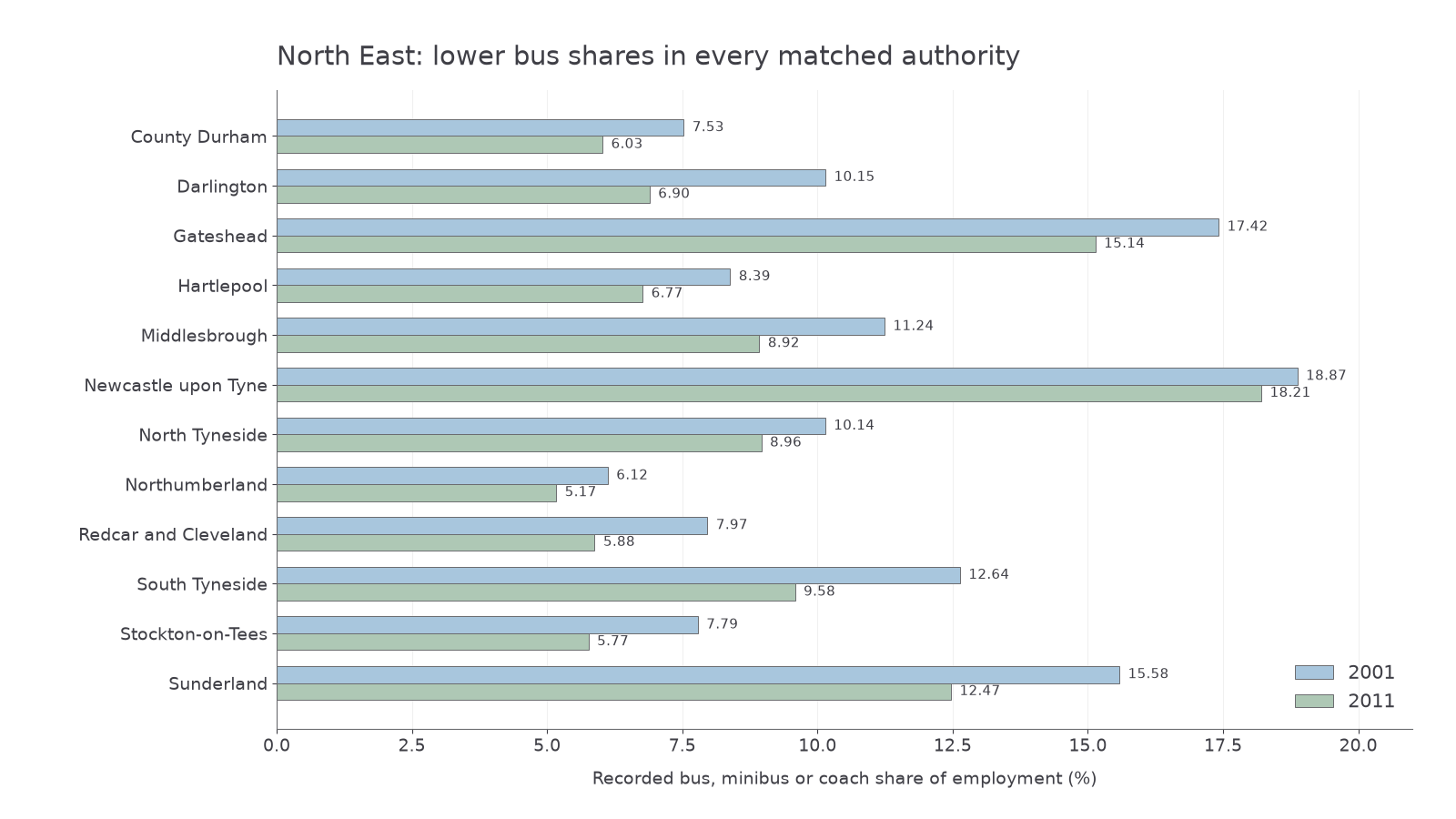
Every authority shown has a lower percentage in . That is a statement about these areas and dates, not a cause or a smooth trend during the intervening decade.
Percentage-point change
For percentages and measured on the same basis,
A relative percentage change instead divides this difference by , then multiplies by . These are different measures. Not in the formula sheet: learn it.
Use unrounded percentages for differences, even when the chart labels show rounded values.
Worked example 3: reading a matched comparison
Question. County Durham's bus percentages were in and in . Calculate the change in percentage points to significant figures and interpret it.
Plan. Subtract the earlier percentage from the later one, then use the sign in the conclusion.
Why this step? The graph compares shares, so the vertical difference is in percentage points, not a relative percentage change.
Answer. The bus percentage decreased by percentage points.
Check. The bar is lower, and the gap is about on the percentage axis.
Change only the authority to Darlington; keep the dates, measure and precision fixed.
Worked example 4: the same graph, another authority
Question. Darlington's bus percentages were in and in . Calculate and interpret the change in percentage points to significant figures.
Plan. Subtract the earlier percentage from the later percentage for this matched pair.
Why this step? Matching areas means a difference reflects a change in that area's recorded share, rather than a difference between two unrelated areas.
Answer. The bus percentage decreased by percentage points.
Check. Darlington's gap is visibly larger than County Durham's.
Other questions need other displays. For an age-structure comparison, divide age-band counts by all usual residents before comparing differently sized authorities. To explore mean age against bus percentage, join the age and travel tables by geography code and create an XY scatter diagram, one complete authority pair per point. Label mean age in years and bus use in percent. Inspect Region groups and unusual points before describing a pooled association; correlation alone would not identify a cause.
Exam tip
Describe what the supplied display actually measures. A lower bus percentage does not establish fewer bus users, because employment may have changed. Two census dates also do not reveal the path between them.
This final matched pair resolves the puzzle at the start.
Continue this lesson.
You’re previewing NovaLearn without an account. Create a free account to read the rest.
Create free account