16.5-16.7 - Rate Graphs And Reaction Orders
Use graph gradients, half-lives and initial-rate ratios to determine reaction orders. Keep the axes, units and controlled variables visible so each conclusion follows from the data.
From A Graph To A Rate
A reaction mixture is monitored every few seconds. The concentration of reactant A falls smoothly, but the graph is not a straight line. Does the reaction have one rate, or does its rate change as the reaction proceeds?
A rate is a change per unit time. On a graph, that means a gradient:
Rate from a graph
= concentration () or volume (); = time (s). For a curve, use the tangent at the required time; the rate of disappearance of a reactant is the positive magnitude of a negative gradient.
The sign and unit come from the graph:
| Graph | Gradient sign | Rate statement usually needed |
|---|---|---|
| Reactant concentration against time | negative | use the positive magnitude for rate of disappearance |
| Product concentration against time | positive | use the positive gradient for rate of appearance |
| Gas volume against time | positive | use the positive gradient for rate of gas production |
If the graph is straight, the rate is constant over that interval. If the graph is curved, the rate at a particular time is found from a tangent at that time. This matters chemically because reactant concentrations change during a run, so the collision frequency and rate often change too.
Use this route:
- Identify the graph and axes.
- Decide whether the question asks for a mean rate, an initial rate, or a rate at a time.
- For a curve, draw a tangent at the required point.
- Choose two well-spaced points on the tangent.
- Calculate the gradient, .
- Use the graph-axis units in the final rate.
Worked example: rate from a concentration-time graph. A tangent to a concentration-time curve at passes through two convenient points:
and
Calculate the rate of disappearance of A at .
The graph gradient is negative because the concentration of A is decreasing. The rate of disappearance of A is the positive magnitude:
The chemical interpretation is that, at about , A is being used up at each second. That is an instantaneous rate, not the mean rate for the whole experiment.
First-Order Half-Life From Graphs
A falling concentration can be compared in fractions as well as absolute changes. Half-life measures the time required for one such fractional change.
Half-life, \(t_{1/2}\)
The time taken for the amount or concentration of a reactant to halve.
For a first-order reaction, successive half-lives are equal at constant temperature.
[DIAGRAM: asset_name: First-order half-life and tangent graph; asset_slug: edexcel_a_level_chemistry_l078_first_order_half_life_tangent; recommended_method: deterministic_chart; description: 16:9 monochrome concentration-time graph for a first-order reaction showing falling from 0.80 to 0.40 to 0.20 to 0.10 mol dm^-3 at equal 30 s intervals, with dashed half-life construction lines and a tangent at 45 s labelled as instantaneous rate.]
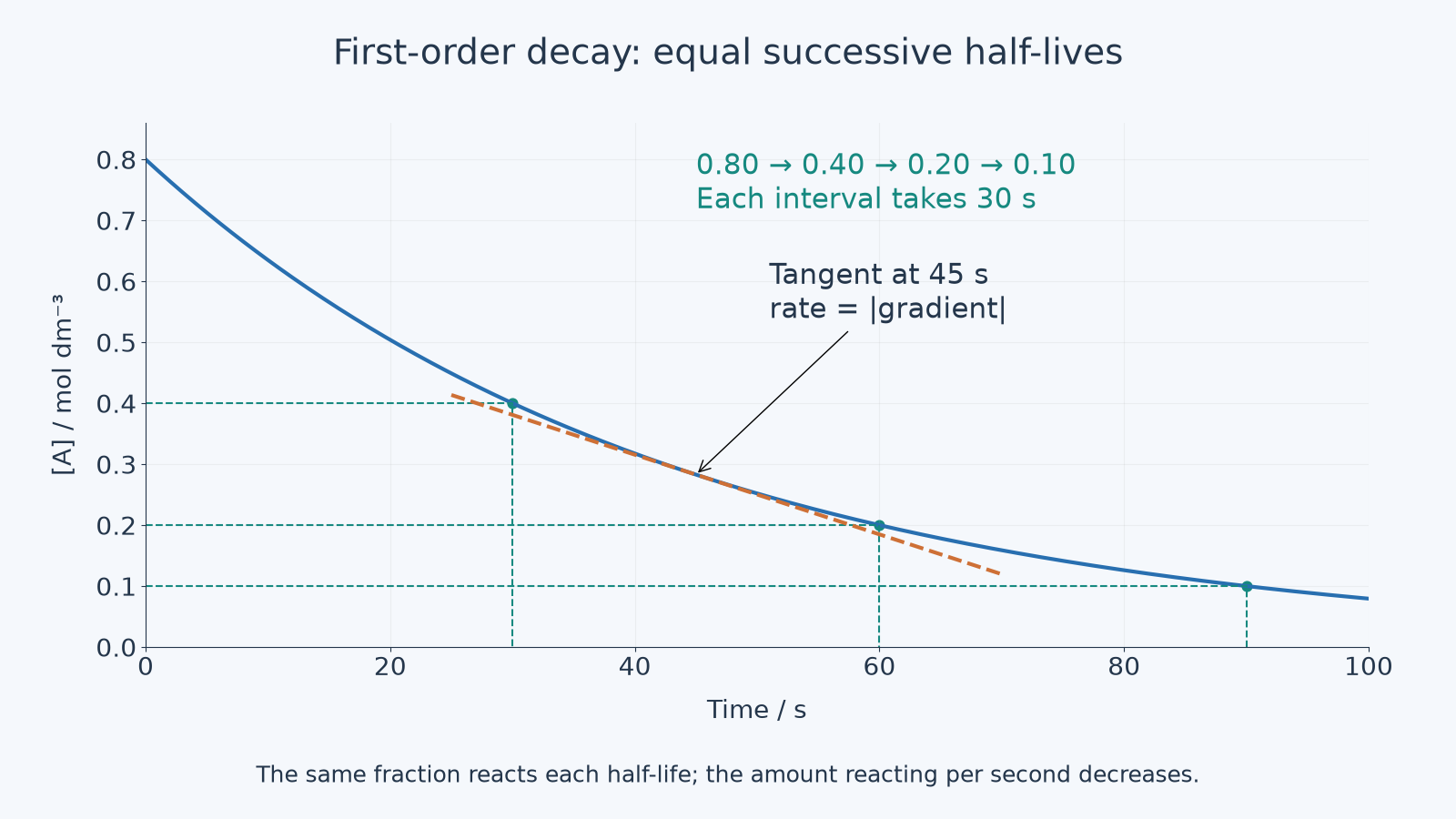
Read a half-life from a concentration-time graph by choosing a concentration and finding the time taken to reach half that concentration. Then repeat from the new concentration. For a first-order reaction, these time intervals should be the same within the accuracy of the graph.
For the graph shown:
- takes 30 s
- takes 30 s
- takes 30 s
So:
Volume-time graphs need one extra thought. A product-volume graph rises towards a final volume. If the gas volume is directly proportional to product formed, and the gas comes from the limiting reactant being used up, then one half-life is the time taken for the product volume to reach halfway to the final volume. The second half-life is the time taken to go from halfway to three-quarters of the final volume, because half of the remaining reactant has reacted.
For a final gas volume of :
- after 1 half-life: product volume
- after 2 half-lives: product volume
- after 3 half-lives: product volume
That sequence is not . The product volume approaches a maximum because the limiting reactant is being used up.
Worked example: half-life from product volume. A first-order decomposition produces gas and reaches a final volume of . The graph shows at and at .
The first value, , is half of the final volume, so it marks one half-life. The second value, , is three-quarters of the final volume, so it marks two half-lives.
first half-life ; second half-life
The half-lives are equal, so the graph is consistent with first-order behaviour in the limiting reactant.
Orders From Concentration-Time Graphs
A concentration-time graph shows how much reactant remains as time passes. To deduce order from this graph, look for the rate pattern, not just whether the line is curved.
[DIAGRAM: asset_name: Graph patterns for reaction order; asset_slug: edexcel_a_level_chemistry_l078_order_graph_patterns; recommended_method: deterministic_chart; description: 16:9 monochrome two-panel chart comparing zero, first and second order evidence; left panel shows concentration-time patterns with zero order as a straight decreasing line, first order as exponential decay with constant half-life markers, and second order as a curve with increasing half-lives; right panel shows rate-concentration patterns with zero order horizontal, first order straight through the origin, and second order upward-curving.]
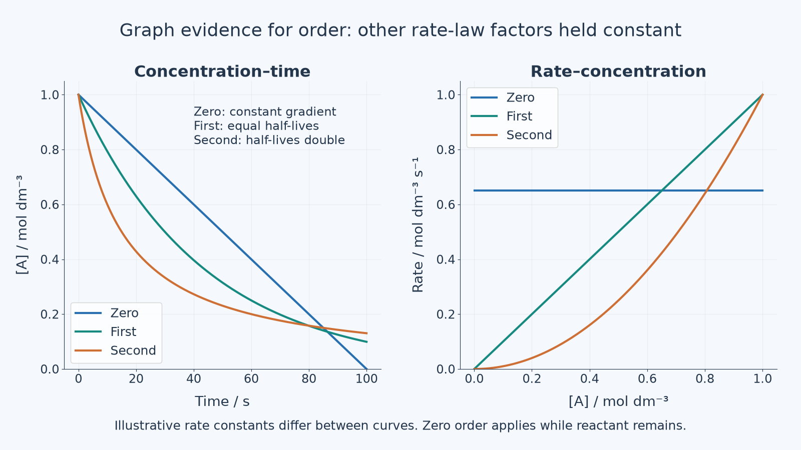
| Order with respect to A | Concentration-time evidence | Chemical meaning |
|---|---|---|
| falls in a straight line; gradient is constant until A is used up | rate does not depend on | |
| falls in a curve with constant successive half-lives | rate is proportional to | |
| falls in a curve, but successive half-lives increase as gets smaller | rate is proportional to |
Zero order is the easiest concentration-time graph to spot: a straight decreasing line means the same amount of A is used up each second. The rate does not fall as falls, so A is zero order under those conditions.
These single-reactant patterns assume other rate-law factors are constant or have been accounted for. If two reactants change substantially during the same run, a curve alone may not isolate the order with respect to one of them.
For a simple second-order decay, successive half-lives double as the concentration halves. Increasing half-lives alone suggest order greater than one; the doubling pattern identifies second order within this model.
First order and second order are both curves, so "it curves" is not enough evidence. For first order, equal half-lives are the key pattern. For second order, the graph flattens in a way that gives longer successive half-lives as concentration decreases.
Continue this lesson.
You’re previewing NovaLearn without an account. Create a free account to read the rest.
Create free account