Q3 - Constant-acceleration equations
Derive and use the equations for motion with constant acceleration along a straight line. You will choose signs consistently, interpret the roots of vertical-motion equations and join stages whose accelerations differ.
Deriving the constant-acceleration equations
If a car doubles its initial speed but brakes with the same constant deceleration, does its stopping distance double? The equations will show why it actually quadruples.
You already know
Velocity–time gradient gives acceleration, and signed area gives displacement. A trapezium has area equal to half the sum of its parallel sides multiplied by their separation. The identity is the difference of two squares.
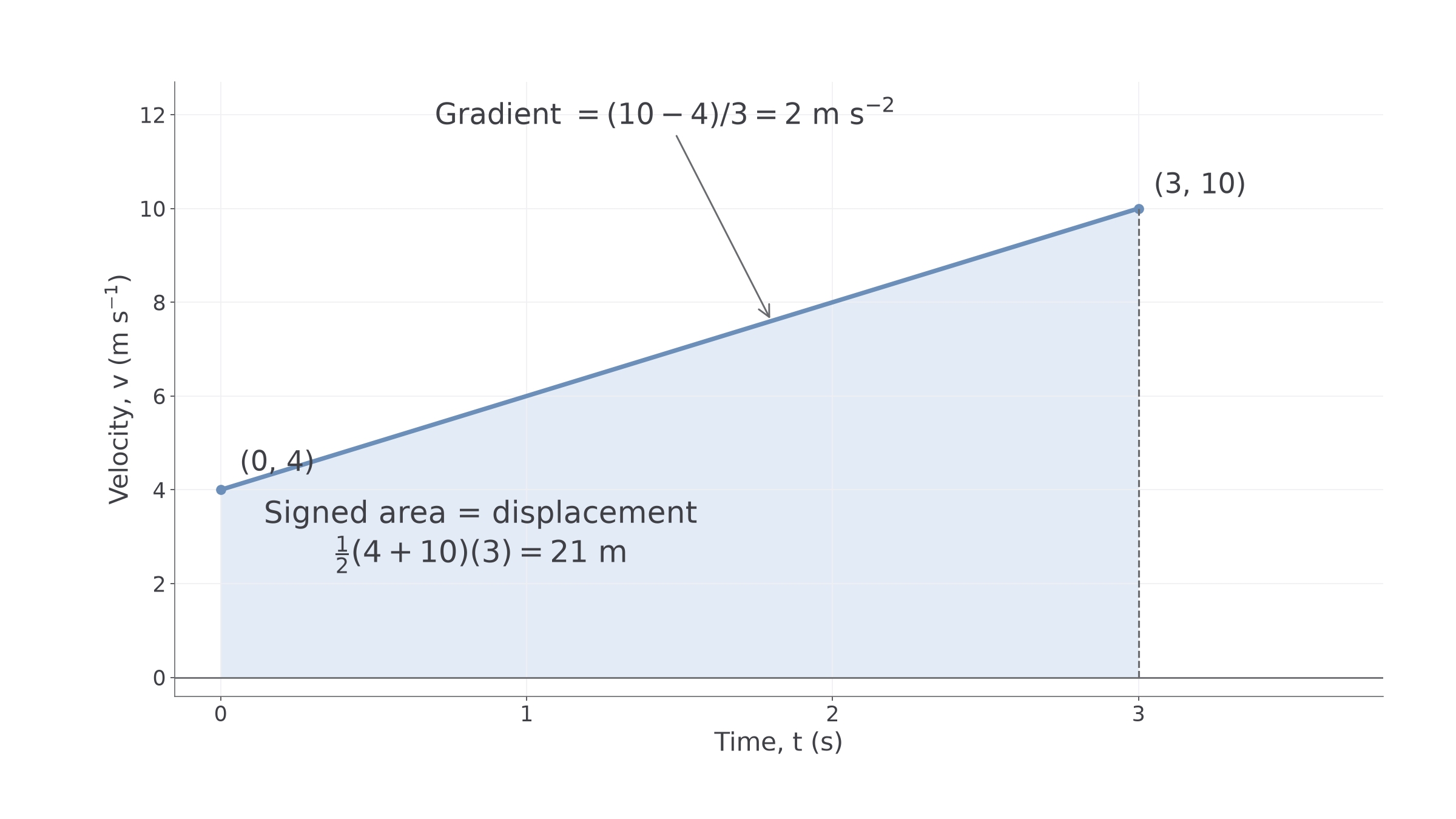
For example, velocity increasing from to in gives acceleration . If this acceleration is constant, the velocity graph is straight and its area is . Without the straight-line condition, its endpoint velocities need not determine the area.
The five motion quantities
Over one interval, is initial velocity, is final velocity, is constant acceleration, is elapsed time and is displacement. In straight-line motion are signed along a chosen axis; elapsed time satisfies . Initial position need not be zero: final position is initial position plus .
Constant acceleration means equal changes of velocity in equal times. The concrete graph below has gradient and area . The same gradient and area reasoning works with letters.
Worked example 1: deriving velocity and displacement
Question. A particle has constant acceleration along a line. Derive and from its velocity–time graph.
Plan. Use the graph's gradient, then use its signed trapezium area and eliminate .
Why this step? Replacing final velocity by expresses displacement using the initial velocity and the constant acceleration.
Answer. The two equations follow from the graph's gradient and area. Both also hold at , when and .
Check. For , , , they give and , agreeing with the concrete graph calculation.
The next derivation changes what is eliminated: remove time instead of final velocity. Avoid dividing by acceleration, so that the argument still includes zero acceleration.
Worked example 2: deriving an equation without time
Question. Starting from and , derive , including the case .
Plan. Multiply the velocity difference by the velocity sum, then replace by .
Why this step? Substitution removes without dividing by , which might be zero.
Answer. , valid for constant acceleration including .
Check. With , both sides equal . If , the original velocity relation gives , consistent with the result.
Eliminating instead gives : substitute into the trapezium area. You now have five equivalent forms for choosing an efficient calculation.
Constant acceleration along a line
For one interval with constant acceleration,
Here is displacement, not automatically distance.
In the formula booklet.
The equations still require the correct interval and signs. A varying-acceleration graph generally has a different area from the straight line joining its endpoints.
Watch out
Wrong: “Every journey has .” Its endpoint average equals average velocity under the constant-acceleration condition, not for an arbitrary velocity curve. Right: establish constant acceleration before using these equations.
Practise a derivation by eliminating the initial rather than final velocity.
Choosing equations and signs
Choose the axis and interval first, then select an equation that omits a quantity you do not need.
For example, avoids time, while avoids final velocity. List the known quantities with their signs and convert to consistent units before substituting. The equations are supplied; the choice of a suitable equation is yours.
Worked example 3: braking until the first stop
Question. A car travels at and has constant acceleration until it first stops. Taking forward as positive, find the stopping time and distance.
Plan. Set , find time from the velocity equation, then find displacement without time.
Why this step? The acceleration is negative along the chosen axis; “braking” does not make its signed value positive.
Answer. The car first stops after , having travelled .
Check. Its velocity remains nonnegative before the stop, so distance equals displacement. The triangular graph area is .
The next interval continues through an instant of rest, so distance can no longer be read directly from the final displacement.
Worked example 4: an interval containing a reversal
Question. A particle has initial velocity and constant acceleration for . Find its final velocity, displacement and distance travelled.
Plan. Use the supplied equations for velocity and displacement, then split the distance where velocity is zero.
Why this step? The final displacement combines two opposite directions; distance needs both travelled legs separately.
Answer. Final velocity is , displacement is , and distance is .
Check. The velocity graph has two triangles: and metres. Their difference is and their sum is .
The opening question now has an exact answer. With forward speed , constant braking magnitude , and final velocity zero, , so stopping distance is . This derived stopping-distance result is not separately printed in the formula booklet; derive it from the supplied equation. Doubling multiplies its square, and hence the stopping distance, by four. At , initial speeds and give and .
Watch out
Wrong: extend example 3 beyond and conclude that the braking car must reverse. The model was stated only until its first stop. Right: end that stage at ; further motion needs further information. A particle explicitly given constant acceleration through a reversal, as in example 4, is a different interval.
Use a new signed interval and split it at its own turning time.
Vertical motion and admissible roots
For vertical motion with constant gravity and no air resistance, acceleration stays downward even when the particle is moving upward or instantaneously at rest.
Take upward as positive, so . A ball launched upward has ; at maximum height ; on descent . The acceleration is still at the top. Treating the ball as a particle, neglecting air resistance and taking as constant are separate assumptions. The constant-acceleration equations are supplied; these modelling decisions are not supplied formulae.
Continue this lesson.
You’re previewing NovaLearn without an account. Create a free account to read the rest.
Create free account