M3 - Probability models and assumptions
Build probability models from clearly defined events and assumptions, then check what their predictions mean. Refine dependence, population weights and physical constraints, and explain how each change affects the answer and what uncertainty remains.
Constructing a probability model
Two pumps each have a chance of failure during a day. Is that enough information to find the chance their system works? You also need to know how the pumps work together and how their failures are related.
A backup system works when at least one pump works. A system requiring both pumps has a different success event, even with exactly the same equipment failure probabilities.
You already know
For independent events, multiply marginal probabilities to find their intersection. In general use a conditional second probability. Complement and addition rules combine the resulting disjoint outcomes.
Before choosing any rule, define one experiment, its population and the time period. Selecting a working day uniformly differs from selecting a repair call: days with many calls contribute more observations to the second experiment.
Probability model
A probability model simplifies a chance process by specifying its possible outcomes or variables, their probabilities and relationships. It must assign nonnegative probabilities totalling , and its assumptions must connect those probabilities to the stated situation.
Equal likelihood supports count-to-total fractions. Independence supports products of marginal probabilities. Stable, representative rates support using past data for a future population. These assumptions are distinct: a constant individual failure rate does not establish independence between pumps.
Worked example 1: a backup arrangement
Question. Each of two pumps fails during a day with probability , independently. A system works if at least one pump works. Construct the four joint-outcome probabilities and find the system's operating probability.
Plan. Define the failure events, form the four disjoint outcomes, then complement total failure.
Let and denote the two failures.
Why this step? A backup arrangement fails only at the intersection of the two failure events.
Answer. The four probabilities are ; the system works with probability .
Check. The four cells sum to , and the three working cells sum to .
Change only the system requirement. The failure probabilities and independence assumption stay the same.
Worked example 2: both pumps required
Question. Two pumps still fail independently with probability each during a day. This system works only if both pumps work. Find its operating and failure probabilities.
Plan. Select the neither-fails cell from the same four-outcome model.
Why this step? The physical arrangement determines whether one failure is enough to stop the system.
Answer. Operating probability ; failure probability .
Check. Failure is , the sum of the other three cells.
These reliability expressions are consequences of the defined system and probability rules; they are not separate formulae in the booklet. The addition and conditional multiplication rules are supplied; independence and complement rules must be learned.
Watch out
Wrong: “Each pump works with probability , so the system works with probability .” An individual pump is not the whole system. Define the system's success event and combine the appropriate outcomes.
A useful assumption criticism names a mechanism. For example, a shared power failure could make the two pump failures dependent.
Refining dependence assumptions
A shared cause can change simultaneous failure without changing either pump's individual failure probability. To refine the model, specify a joint or conditional probability that expresses this relationship. Saying only “dependent” does not tell you which way the answer changes.
For the backup pumps, retain . Write . The four cells must then be . Nonnegativity requires , and the system's operating probability is , between and . Those are derived bounds, not supplied booklet formulae.
This is a striking limitation of the original information: two -reliable pumps can give a backup operating probability anywhere from to , depending on their relationship. Under independence it is ; that value is one model, rather than a consequence of the two individual rates alone.
Worked example 3: more simultaneous failures
Question. For the backup system, retain , but set . Find the four joint cells, , and the system's operating probability. Compare with independence.
Plan. Subtract the overlap from each marginal, complete the table and condition on the appropriate row.
Why this step? The overlap fixes both conditional branches; retaining on them would contradict the refined joint model.
Answer. Cells ; conditionals and ; operating probability , down from .
Check. The cells sum to and both failure margins remain .
The comparison is visible in the two complete tables: the common-failure cell grows while each failure margin stays fixed.
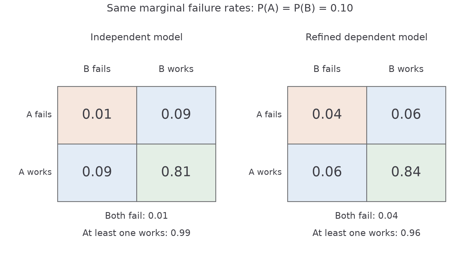
Change only the overlap to . Dependence can also reduce simultaneous failure.
Worked example 4: fewer simultaneous failures
Question. The same backup pumps have failure probabilities each, now with . Find the four cells, the two B-failure conditional probabilities and the operating probability. Compare with independence.
Plan. Use the same cell construction with the new overlap.
Why this step? The operating event is still the complement of both failures; its change follows the specified overlap, rather than the word “dependent”.
Answer. Cells ; conditionals and ; operating probability , above .
Check. Each failure margin is , and explains the gain over independence.
At the extremes, means simultaneous failure has probability zero, while means the two failure statuses agree with probability one. Neither conclusion follows merely from equal marginal rates.
Watch out
Wrong: “Dependence always lowers backup reliability.” In example 4, the overlap is below the independent value, so reliability rises. State how the refined relationship changes the particular failure event.
Before interpreting any refinement, check that its cells are valid probabilities.
Continue this lesson.
You’re previewing NovaLearn without an account. Create a free account to read the rest.
Create free account