N2 - Normal distributions and probabilities | AQA A-Level Mathematics

Use a Normal curve to model continuous measurements, calculate probabilities and find cutoffs. You will connect the curve's shape to its parameters, recover unknown parameters from probability information, and use one measurement's probability in a binomial count.

Normal shape and parameters

Two machines fill packets to the same average mass. Can their curves have the same centre but different heights and spreads? Imagine one machine producing very similar masses and another varying much more. The second curve must spread its probability over a wider interval, so its peak is lower.

You already know

A histogram's bar area represents frequency; after scaling to relative frequency, total area is $1$ . Standard deviation measures spread in the original units, while variance is its square. An inflection point is where a curve changes concavity.

A roughly symmetric histogram with one mound may suggest a Normal model. Symmetry alone is insufficient: two peaks can also be symmetric. Class widths and sample size affect what a histogram reveals.

Normal distribution

$X\sim \mathrm N(\mu,\sigma^2)$ denotes a Normal distribution with population mean $\mathrm E(X)=\mu$ , variance $\operatorname{Var}(X)=\sigma^2$ and standard deviation $\sigma>0$ . Its bell-shaped density is symmetric about $\mu$ , with total area $1$ .

The second parameter is variance. The model allows every real value; distant values can have extremely small probabilities. A density height is not itself a probability: probability is area. A wider Normal curve has a lower peak because its area remains $1$ . These shape and parameter facts are not in the formula booklet: learn them.

Why the inflections reveal the standard deviation

A Normal curve changes concavity at $\mu-\sigma$ and $\mu+\sigma$ . You need to understand and be able to show this. If a calculus question requires the density, the needed equation is supplied; it is not in the formula booklet and you need not memorise it. Starting from a supplied equation

f(x)=C\exp\!\left(-\frac{(x-\mu)^2}{2\sigma^2}\right),\qquad C>0,\ \sigma>0

treat $C,\mu,\sigma$ as constants. The chain rule gives

f'(x)=-\frac{x-\mu}{\sigma^2}f(x)

Then the product rule gives

\begin{aligned} f''(x)&=-\frac1{\sigma^2}f(x)-\frac{x-\mu}{\sigma^2}f'(x) && \text{differentiate both factors} \\ &=-\frac1{\sigma^2}f(x)+\frac{(x-\mu)^2}{\sigma^4}f(x) && \text{substitute }f'(x) \\ &=\frac{f(x)}{\sigma^4}\bigl((x-\mu)^2-\sigma^2\bigr) && \text{factorise} \end{aligned}

The factor $f(x)/\sigma^4$ is positive. The bracket is positive outside $(\mu-\sigma,\mu+\sigma)$ and negative inside it. Thus $f''$ changes sign at both endpoints, establishing both inflections. Merely solving $f''=0$ would not establish a change of concavity. This derivation and the inflection locations are not in the formula booklet: learn the reasoning.

Worked example 1: reading the scale of a curve

Question. For $X\sim \mathrm N(80,16)$ , state the mean and standard deviation, locate the inflections and give the interval within three standard deviations of the mean.

Plan. Take the square root of the second parameter before measuring distances from the centre.

\begin{aligned} \mu&=80,\qquad\sigma=\sqrt{16}=4 && \text{second parameter is variance} \\ \mu-\sigma&=76,\qquad\mu+\sigma=84 && \text{inflection locations} \\ \mu-3\sigma&=68,\qquad\mu+3\sigma=92 && \text{three-SD limits} \end{aligned}

Why this step? The horizontal distance to an inflection is one standard deviation, rather than one variance.

Answer. Mean $80$ , standard deviation $4$ , inflections at $76,84$ , and three-SD interval $[68,92]$ .

Check. Both inflections are $4$ from the centre, and the interval is centred on $80$ .

Change only the variance from $16$ to $64$ . The mean stays fixed, while all distances measured in standard deviations double.

Worked example 2: a wider curve with the same centre

Question. For $Y\sim \mathrm N(80,64)$ , find the same quantities.

Plan. Recalculate $\sigma$ , then use the same centre-and-distance method.

\begin{aligned} \mu&=80,\qquad\sigma=\sqrt{64}=8 && \text{new standard deviation} \\ \mu\pm\sigma&=80\pm8 && \text{inflection locations} \\ \mu\pm3\sigma&=80\pm24 && \text{three-SD limits} \end{aligned}

Why this step? Quadrupling variance doubles standard deviation; it does not quadruple horizontal distances.

Answer. Mean $80$ , standard deviation $8$ , inflections at $72,88$ , and three-SD interval $[56,104]$ .

Check. Each interval is twice as wide as in Worked example 1, with the same centre.

The first curve shows how the inflections mark its scale.

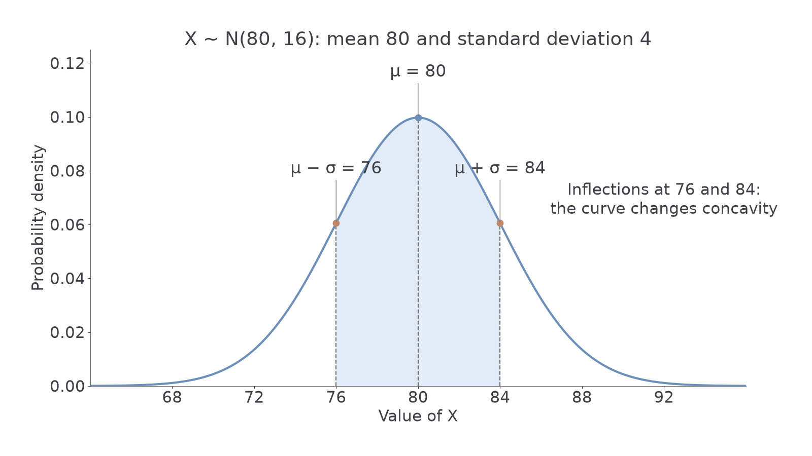
Normal density centred at 80, with inflections at 76 and 84 and the one-standard-deviation interval shaded

Approximately $68.3\%$ , $95.4\%$ and $99.7\%$ of any Normal distribution lie within one, two and three standard deviations of its mean. These are useful recall facts, not printed formulae. Remarkably, changing the mean or spread leaves those proportions unchanged. Standardisation in the next part explains why.

Watch out

Wrong: $\mathrm N(80,16)$ has standard deviation $16$ and inflections at $64,96$ . The second parameter is variance. Right: $\sigma=4$ , so the inflections are $76,84$ .

A fitted smooth curve can suggest approximate mean and standard deviation from its centre and inflections. An irregular histogram does not supply exact inflection locations. Apply the parameter interpretation to a mass model.

Normal probabilities and standardisation

A packet mass can fall anywhere in an interval. Describe that interval or tail first, then calculate its area using the model's mean and standard deviation.

Because a point has no area, $\mathrm P(X=a)=0$ for a continuous Normal variable. Consequently strict and inclusive endpoints have the same probability: for example, $\mathrm P(X<a)=\mathrm P(X\leq a)$ . A mass recorded as $500\,\mathrm g$ after rounding is different: it represents an interval of true masses, which can have positive probability.

Individual standardisation

For $X\sim \mathrm N(\mu,\sigma^2)$ ,

Z=\frac{X-\mu}{\sigma}\sim \mathrm N(0,1),\qquad z=\frac{x-\mu}{\sigma}

Not in the formula booklet: learn it.

A z-score measures how many standard deviations a value lies to the right of the mean. Negative scores lie below the mean. Subtracting the mean centres the variable; dividing by positive $\sigma$ removes its scale and preserves inequalities. All Normal models therefore give the same probabilities between corresponding z-scores. This explains the common central proportions above.

Write $\phi(z)$ for standard Normal density and $\Phi(z)=\mathrm P(Z\leq z)$ for lower-tail probability. By symmetry, $\Phi(-z)=1-\Phi(z)$ and $\Phi(0)=0.5$ . These identities are not printed in the formula booklet: learn them. Do not confuse density $\phi$ with area $\Phi$ .

Use the calculator's Normal probability function directly: enter lower bound, upper bound, mean and standard deviation. For a tail, use its supported infinite-bound convention. If it gives cumulative lower-tail probabilities, take a complement for an upper tail or subtract two values for an interval. The Mathematics formula booklet contains no statistical tables.

Worked example 3: an interval and its two tails

Question. Fill mass $W$ , in grams, has model $W\sim \mathrm N(500,6^2)$ . Find $\mathrm P(W<494)$ , $\mathrm P(W>509)$ and $\mathrm P(494<W<509)$ , to four decimal places.

Plan. Standardise both boundaries to check the calculator's areas.

\begin{aligned} z_{494}&=\frac{494-500}{6}=-1 && \text{one SD below} \\ z_{509}&=\frac{509-500}{6}=1.5 && \text{one and a half SD above} \\ \mathrm P(W<494)&=\Phi(-1)=0.1586552539\ldots && \text{lower tail} \\ \mathrm P(W>509)&=1-\Phi(1.5)=0.0668072013\ldots && \text{upper tail} \\ \mathrm P(494<W<509)&=\Phi(1.5)-\Phi(-1) && \text{between the boundaries} \\ &=0.7745375448\ldots && \text{calculator evaluation} \end{aligned}

Why this step? The upper-tail probability uses the complement of the area below $509$ .

Answer. Respectively $0.1587$ , $0.0668$ and $0.7745$ .

Check. The three unrounded probabilities total $1$ .

Change only the upper boundary from $509$ to $512$ . The lower tail stays the same, while the middle interval grows.

Worked example 4: moving one boundary

Question. For the same mass model, find $\mathrm P(W<494)$ , $\mathrm P(W>512)$ and $\mathrm P(494<W<512)$ , to four decimal places.

Plan. Keep the lower z-score and standardise the new upper bound.

\begin{aligned} z_{512}&=\frac{512-500}{6}=2 && \text{new upper score} \\ \mathrm P(W<494)&=\Phi(-1)=0.1586552539\ldots && \text{unchanged lower bound} \\ \mathrm P(W>512)&=1-\Phi(2)=0.0227501319\ldots && \text{smaller upper tail} \\ \mathrm P(494<W<512)&=\Phi(2)-\Phi(-1) && \text{interval area} \\ &=0.8185946141\ldots && \text{evaluate} \end{aligned}

Why this step? Moving the upper bound right transfers area from the upper tail to the interval.

Answer. Respectively $0.1587$ , $0.0228$ and $0.8186$ .

Check. The interval probability exceeds $0.7745$ , and the three unrounded probabilities still total $1$ .

For a simpler symmetry check, $X\sim \mathrm N(12,9)$ gives $\mathrm P(X\geq12)=\mathrm P(X>12)=0.5$ : the exact centre has probability zero.

Watch out

Wrong: enter $36$ as the standard deviation for $\mathrm N(500,36)$ . Right: enter $6$ . The model notation uses variance, but the probability calculator normally asks for its square root.

Your next interval has the same sort of unequal distances from the mean, in a new measurement model.

Inverse Normal cutoffs

Sometimes the probability is known and the boundary is missing. A quantile $a$ with lower-tail probability $u$ satisfies $\mathrm P(X\leq a)=u$ . An inverse Normal function reverses a cumulative calculation.

For $0<u<1$ , find $z=\Phi^{-1}(u)$ , then rearrange standardisation to obtain $a=\mu+\sigma z$ . This rearrangement is not in the formula booklet: learn it. A calculator can also return $a$ directly from the left area, mean and standard deviation. Check which tail its inverse function uses.

Continue this lesson.

You’re previewing NovaLearn without an account. Create a free account to read the rest.

Create free account

Last Accessed

Pure Mathematics

Mechanics

Statistics

N2 - Normal distributions and probabilities

Normal shape and parameters

Why the inflections reveal the standard deviation

Normal probabilities and standardisation

Inverse Normal cutoffs

Continue this lesson.

Learn faster with Nova