O1 - Correlation hypothesis tests
Interpret a supplied correlation coefficient and test for population linear correlation using a supplied critical value or p-value. Learn why strength, significance and causation answer different questions, and state what the evidence can reasonably support.
Correlation measures straight-line closeness
Can a sample coefficient of accompany a perfectly predictable relationship? Yes: a U-shaped pattern can have no overall linear direction. A correlation coefficient measures closeness to a straight line, so the shape of the relationship matters.
For example, the paired values with and have supplied coefficient . Each positive has a matching negative with the same . Their upward and downward linear contributions cancel, even though knowing determines exactly.
You already know
A scatter diagram shows paired quantitative observations. Positive correlation means larger values tend to occur together; negative correlation means larger values of one variable tend to accompany smaller values of the other. A hypothesis test uses a sample to investigate a population claim, with a stated risk of incorrect rejection.
Use a plot to check the shape before interpreting a single summary number. An outlier can also have a large influence on a coefficient.
Sample and population correlation
The sample product moment correlation coefficient, , measures the direction and closeness to a straight line in observed paired data. The population correlation coefficient, , describes population linear correlation. Both lie between and . A magnitude of represents exact straight-line alignment; zero represents no linear correlation, rather than no possible relationship.
The sign gives direction; the magnitude gives closeness to a line. Thus represents closer alignment than , because . A negative number is not automatically a weak correlation. Nor is a gradient: converting a length from metres to centimetres changes a graph's gradient but leaves its correlation coefficient unchanged. These interpretations are not in the formula booklet: learn them.
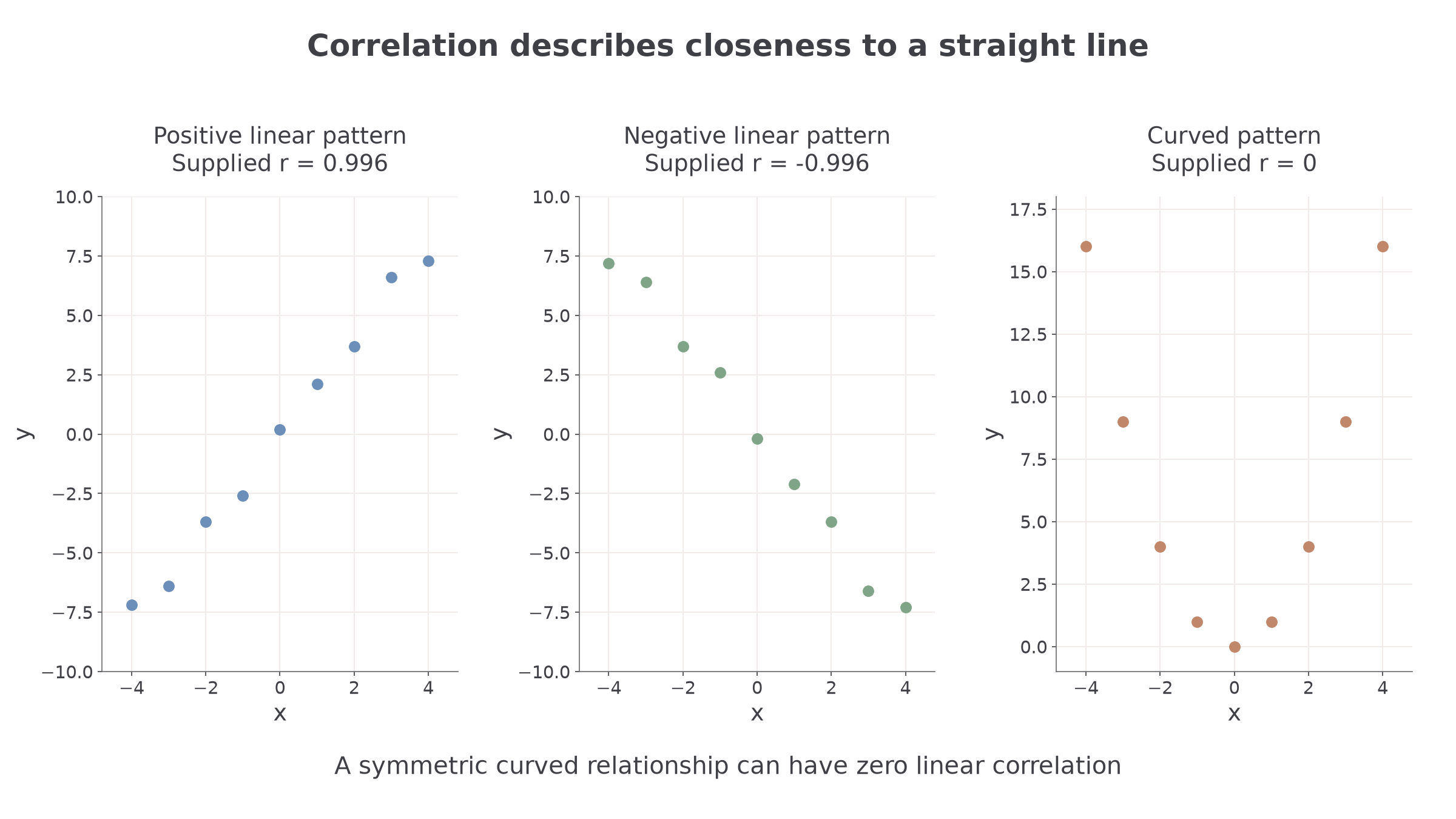
The third panel answers the opening puzzle visually. It has a relationship, but a straight line cannot describe its U shape. Zero correlation therefore does not establish independence. For this course, correlation coefficients are given; you do not need a method for calculating them.
Key idea
Read the sign as direction and the magnitude as straight-line closeness. A coefficient does not describe every kind of relationship.
The next question separates linear strength from the direction of the relationship.
Hypotheses about population correlation
A sample coefficient usually differs from zero even when the population has no linear correlation. The test asks whether the observed coefficient is sufficiently unusual under the population claim .
Write hypotheses using , rather than the already observed . As with a proportion test, choose the direction from the investigation before seeing the sample.
| Investigative claim | Hypotheses | Relevant direction |
|---|---|---|
| Positive population linear correlation | , | Large positive |
| Negative population linear correlation | , | Large negative in magnitude |
| Population linear correlation in either direction | , | Large $ |
These hypothesis conventions are not in the formula booklet: learn them. The exact null distribution used for the usual PMCC test assumes that paired observations form an independent random sample from a bivariate Normal population. This means a joint Normal model for the two variables; it is stronger than merely having two separate bell-shaped histograms. You need to state or assess the assumption, not calculate a bivariate density.
Repeated measurements from the same person may be dependent. A volunteer sample may fail to represent the intended population. A numerical comparison can still be performed, but those weaknesses limit the resulting inference.
Worked example 1: a negative direction
Question. A researcher investigates whether students with longer journeys to school tend to sleep for fewer hours. Define the parameter, state hypotheses and name the distribution assumption for the usual PMCC test.
Plan. Name the population relationship, then translate “longer journey, less sleep” into its sign.
Why use ? The claim concerns all students in the intended population; only describes the observed sample.
Answer. Use a negative one-tailed test of against , assuming an independent random sample of pairs from a bivariate Normal population.
Check. Larger journey durations paired with smaller sleep durations describe negative, rather than positive, linear correlation.
Example 2 changes only the investigative claim. There is now no predicted direction, so both tails matter.
Worked example 2: either direction
Question. The researcher instead investigates whether journey duration and sleep duration have population linear correlation in either direction. State the parameter, hypotheses and model assumption.
Plan. Keep the same population coefficient, but allow either sign in the alternative.
Why is the alternative not a sample coefficient? It specifies which population departures count as evidence before the sample is observed.
Answer. Use a two-tailed test, with the same independent random sampling and bivariate Normal assumptions.
Check. Both and satisfy the alternative; zero does not.
The sample coefficient determines the evidence, not the value to put into a population alternative.
Watch out
Wrong: after observing , write , . The first error uses a sample statistic in population hypotheses; the second makes the alternative an observed exact value. Right, for a pre-specified negative test: , .
Use the purpose of the study to correct the following positive-tail test.
Using supplied critical values and p-values
A critical value tells you how far the sample coefficient must lie from zero for rejection. Use the value supplied for the sample size, significance level and tail. There is no universal cutoff such as .
The Mathematics formula booklet has no statistical tables. AQA supplies the required critical value, a relevant extract, or a p-value. Do not calculate a PMCC or introduce an additional test statistic. The comparison rules themselves are not in the formula booklet: learn them.
For a positive one-tailed test, reject for sufficiently large positive . For a negative one-tailed test, reject for sufficiently negative . If a positive critical magnitude is supplied for that negative test, its signed boundary is . For a two-tailed test, compare with the supplied two-tailed critical magnitude.
Continue this lesson.
You’re previewing NovaLearn without an account. Create a free account to read the rest.
Create free account