C4 - Parametric models | AQA A-Level Mathematics

Construct and use models with a shared parameter, interpret their outputs and valid intervals, and check when observations require a model to change. You will distinguish a geometric path crossing from two objects occupying the same place at the same time.

Constructing shared-parameter models

If two moving objects have paths that cross, must they collide? To answer, you need more than the paths: you need their positions at a common time. Begin with a drone at map position $(2,5)$ metres. If its coordinates change by $3$ and $-2$ metres each second, then two seconds later it is at $(8,1)$ .

You already know

A parametric description uses one input in both equations. A constant-rate model has an initial value and a change per input unit. Eliminating the parameter gives a relation between outputs, but usually loses timing information.

Define every variable, unit, origin and valid interval before interpreting a result. A negative map coordinate means a position on the negative side of the origin, rather than a negative distance travelled.

A constant-rate component

If a quantity starts at $q_0$ and changes at constant rate $k$ , its model is

q=q_0+kt

The units of $k$ are quantity units per parameter unit. The rate must remain constant over the stated interval.

Not in the formula booklet: learn it.

For two quantities, give both equations the same parameter and interval. It need not represent motion: output and cost can share a machine's operating time.

Worked example 1: position on a map

Question. A drone starts at $(2,5)$ metres. For the next three seconds, its horizontal map coordinate increases at $3\,\mathrm{m\,s^{-1}}$ and its vertical map coordinate decreases at $2\,\mathrm{m\,s^{-1}}$ . Construct the model and find its positions after two and three seconds.

Plan. Add each constant rate times elapsed time to its starting coordinate.

\begin{aligned} x&=2+3t && \text{initial horizontal coordinate and rate} \\ y&=5-2t && \text{decreasing vertical map coordinate} \\ t=2&:\quad (x,y)=(8,1) && \text{substitute the same time} \\ t=3&:\quad (x,y)=(11,-1) && \text{end of the stated interval} \end{aligned}

Why this step? Both coordinates must describe the same instant; mixing two times would invent a position.

Answer. $x=2+3t,\ y=5-2t,\ 0\le t\le3$ , with coordinates in metres and $t$ in seconds. The positions are $(8,1)$ and $(11,-1)$ .

Check. At $t=0$ the model gives $(2,5)$ ; in each second the changes are exactly $3$ and $-2$ metres.

The next example changes the interpretation of the two outputs. The shared parameter still connects them, although the resulting curve is not a physical path.

Worked example 2: output and cost

Question. A machine operates for $0\le h\le4$ hours. It produces $2\,\mathrm{m^2}$ of material per hour, starts with zero output, and costs £60 to start plus £35 per operating hour. Find models for output $A$ and cost $C$ , eliminate $h$ , and find both outputs after three hours.

Plan. Model each quantity in terms of hours, then use the output equation to replace $h$ .

\begin{aligned} A&=2h && \text{constant production rate} \\ C&=60+35h && \text{fixed and running costs} \\ h&=\frac A2 && \text{rearrange the output model} \\ C&=60+17.5A && \text{eliminate operating time} \\ h=3&:\quad A=6,\quad C=165 && \text{evaluate both outputs} \end{aligned}

Why this step? Dividing the hourly cost rate by the hourly output rate gives the running cost per square metre.

Answer. $A=2h,\ C=60+35h$ , $0\le h\le4$ . Equivalently $C=60+17.5A$ , $0\le A\le8$ , with $A$ in square metres and $C$ in pounds. At three hours the output is $6\,\mathrm{m^2}$ and cost is £165.

Check. $60+17.5(6)=165$ , agreeing with the time model.

Both models assume steady rates without downtime, discounts or changing conditions. Two matching observations can fit the rates; they cannot establish those assumptions for all possible times.

Watch out

Wrong: a negative $y$ in a map model means an impossible negative height. Right: first read the variable definition. A map coordinate may be negative; height above an impenetrable ground surface cannot be.

For the next machine, change the rates and fixed charge while keeping the shared-time construction.

Trajectories and valid time intervals

A curved path model stops at the event that ends the motion being described, even if the algebra accepts later inputs.

For a ball released above level ground, solve $y=0$ to find a possible impact time. A root before release is outside the model, and a later below-ground continuation needs an impact or bounce model. The trajectory is the spatial path followed by the object.

Valid time interval

A valid time interval contains the times for which the assumptions and contextual conditions of the model apply. For a model beginning at release and ending at first ground contact, include release and that contact, then stop. A real algebraic root before release is not a later landing.

The following flight equations are given models. Their downward quadratic terms represent a constant downward acceleration; the mechanical derivation comes later. Assume level ground, uniform gravity and negligible air resistance. Constant-acceleration formulae are in the booklet, but choosing the contextual interval, eliminating time and completing a square to find a maximum are not supplied as formulae: learn these methods.

Worked example 3: a flight from ground level

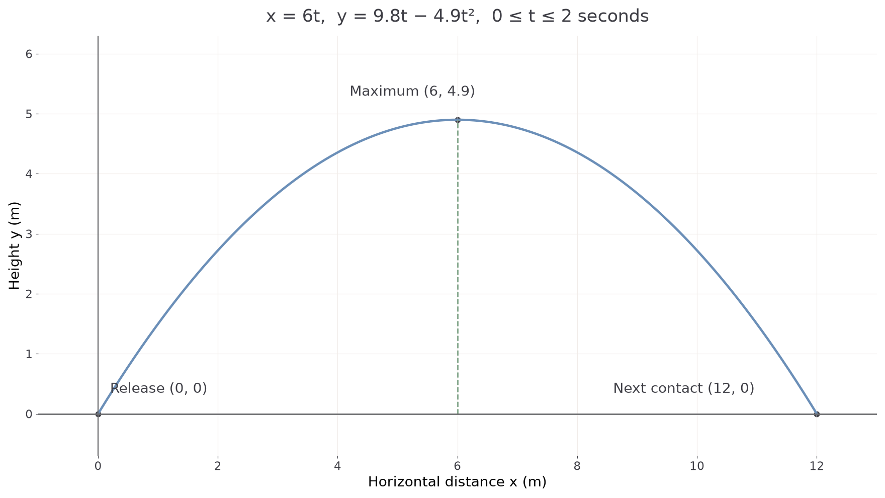
Question. A ball follows $x=6t,\ y=9.8t-4.9t^2$ , with distances in metres and $t$ seconds after release. The model stops at its next ground contact. Find its valid time interval, landing position, maximum height and Cartesian trajectory.

Plan. Solve $y=0$ , complete the time-square for the maximum, and replace $t$ by $x/6$ .

\begin{aligned} 0&=4.9t(2-t) && \text{ground contact} \\ t&=0\text{ or }2 && \text{release or return} \\ y&=4.9-4.9(t-1)^2 && \text{complete the square} \\ t&=\frac x6 && \text{eliminate time} \\ y&=\frac{49}{30}x-\frac{49}{360}x^2 && \text{substitute} \end{aligned}

Why this step? The larger ground root ends this flight; the earlier root is the release event.

Answer. $0\le t\le2$ . Landing is at $(12,0)$ . Maximum height is $4.9\,\mathrm m$ at $t=1$ , with $x=6$ . The displayed Cartesian equation has $0\le x\le12$ .

Check. The square is nonnegative, so $y\le4.9$ , with equality at the allowed time $1$ . The Cartesian equation gives zero at both $x=0$ and $x=12$ .

The diagram ends at the next ground contact; extending the parabola would add points outside this flight.

The ball rises from (0, 0) to (6, 4.9), then lands at (12, 0)

The next example changes only the launch height. One ground root now lies before release and must be rejected.

Worked example 4: release above the ground

Question. A ball follows $x=6t,\ y=4.9+9.8t-4.9t^2$ , from $t=0$ until first ground contact. Find its valid interval, landing position and maximum height.

Plan. Complete the square to obtain both the ground times and maximum, then apply $t\ge0$ .

\begin{aligned} y&=9.8-4.9(t-1)^2 && \text{complete the square} \\ 0&=9.8-4.9(t-1)^2 && \text{ground contact} \\ (t-1)^2&=2 && \text{rearrange} \\ t&=1\pm\sqrt2 && \text{both algebraic roots} \end{aligned}

Why this step? Since $1-\sqrt2<0$ , only the other root is a future event after the model's start.

Answer. $0\le t\le1+\sqrt2$ . Landing is at $(6+6\sqrt2,0)$ metres. Maximum height is $9.8\,\mathrm m$ at $t=1$ , which lies in the valid interval.

Check. At release, $y=9.8-4.9=4.9$ . At $t=1+\sqrt2$ , $y=9.8-4.9(2)=0$ .

A height below the maximum can occur twice, on ascent and descent. Keep both roots if both lie in the valid interval and the question asks for every time.

Watch out

Wrong: choose every real root of $y=0$ as a landing time. Right: identify release, reject pre-release roots, and select the first later ground contact.

The next flight changes the coefficients. Its maximum can still be found from a completed square, without calculus.

Path crossings and common time

Two paths crossing at a point does not establish that two objects reach it together: a collision requires a common position at a common time.

Use a clock measured from the same starting instant. For point-like objects $A,B$ , solve both $x_A(t)=x_B(t)$ and $y_A(t)=y_B(t)$ at the same allowed $t$ . A geometric path intersection instead permits separate parameters, one for each path. These criteria are not in the formula booklet: learn the distinction.

Worked example 5: paths cross without collision

Question. Two robots share a clock. Their map positions are $A:x=2t,\ y=1+t$ and $B:x=6-t,\ y=4$ , for $0\le t\le4$ , with metres and seconds. Show that their paths cross, and determine whether they collide.

Plan. Locate the geometric crossing, then test equality of coordinates using one common time.

\begin{aligned} 1+t_A&=4 && A\text{ reaches the horizontal path} \\ t_A&=3,\quad (x_A,y_A)=(6,4) && \text{crossing point} \\ 6-t_B&=6 && B\text{ reaches that point} \\ t_B&=0 && \text{a different time} \\ 2t&=6-t && \text{common horizontal position} \\ t&=2,\quad y_A=3,\quad y_B=4 && \text{test the only candidate} \end{aligned}

Why this step? Separate arrival times prove a geometric crossing; a collision needs both equations to hold at one time.

Answer. The paths cross at $(6,4)$ , but there is no collision: the only possible common- $x$ time has different $y$ coordinates.

Check. At the path-crossing time $t=3$ for $A$ , robot $B$ is at $(3,4)$ , not $(6,4)$ .

The paths cross exactly, yet the robots never meet: timing changes the outcome. The equations above prove it by exhausting the only common- $x$ candidate.

The next example changes only robot $B$ 's constant $y$ coordinate, from $4$ to $3$ . That is enough to change the collision conclusion.

Worked example 6: a common position and time

Question. Now $A:x=2t,\ y=1+t$ and $B:x=6-t,\ y=3$ , for $0\le t\le4$ . Determine whether they collide.

Plan. Find the common- $x$ candidate and check the other coordinate at that same time.

\begin{aligned} 2t&=6-t && \text{equal horizontal coordinates} \\ t&=2 && \text{only candidate} \\ y_A(2)&=1+2=3 && \text{first vertical coordinate} \\ y_B(2)&=3 && \text{second vertical coordinate} \\ x_A(2)=x_B(2)&=4 && \text{common horizontal coordinate} \end{aligned}

Why this step? A candidate from one coordinate becomes a collision only after the other coordinate and the valid interval both agree.

Answer. They collide at $t=2$ seconds, at $(4,3)$ metres.

Check. Direct substitution into both original models gives $(4,3)$ , and $2\in[0,4]$ .

If one clock starts later, first translate both equations to a common clock. Also, real objects have size: distinct modelled centres do not establish a safe clearance for finite robots.

Watch out

Wrong: $x_A=x_B$ proves a collision. Right: it supplies candidate times only; check $y_A=y_B$ at each of them and reject times outside the shared model interval.

The next pair changes the rates and starting positions. The collision criterion stays the same.

Checking and refining models

Compare a prediction with observations and their uncertainty before deciding which assumption to change.

A discrepancy might reflect measurement error, incorrect parameter values or a changing rate. Refinement should target the failed part of the model, then be checked using further observations. Fitting an observation is not an independent test of the fit.

Prediction discrepancy

A prediction discrepancy is the difference between a prediction and an observation. Compare its size with the stated measurement uncertainty. For example, an observation of $10.4\,\mathrm m$ with uncertainty $0.1\,\mathrm m$ represents the interval $[10.3,10.5]\,\mathrm m$ , not exact agreement with $10.4$ alone.

To refit a constant rate while retaining a starting value $q_0$ , solve $q_{\text{observed}}=q_0+kt$ . This fitting method is not in the formula booklet: learn the reasoning. It changes a parameter, rather than proving that the constant-rate assumption is correct.

Worked example 7: refining a horizontal rate

Question. The drone model $x=2+3t,\ y=5-2t$ , $0\le t\le3$ , predicts metres after $t$ seconds. At $t=3$ , a reliable observation is $x=10.4\,\mathrm m$ , with uncertainty $0.1\,\mathrm m$ , and $y=-1\,\mathrm m$ . Assess the prediction and refit the constant horizontal rate, keeping the starting point.

Plan. Compare the prediction with the uncertainty interval, then fit $x=2+ut$ to the central observation.

\begin{aligned} x(3)&=2+3(3)=11 && \text{original prediction} \\ 10.3\le x_{\text{observed}}&\le10.5 && \text{measurement interval} \\ 10.4&=2+3u && \text{fit the retained start} \\ u&=2.8 && \text{new horizontal rate} \end{aligned}

Why this step? The stated uncertainty does not reach $11$ , so it cannot alone explain the original discrepancy.

Answer. The original horizontal prediction is inconsistent with that uncertainty. A refined model is $x=2+2.8t,\ y=5-2t,\ 0\le t\le3$ . The observed vertical coordinate matches the original, so there is no evidence here to change that component.

Check. The revised model gives $x(3)=10.4$ , keeps $x(0)=2$ , and predicts $(4.8,3)$ at $t=1$ , $(7.6,1)$ at $t=2$ .

The next example changes only the observation to one compatible with the original prediction. A central reading need not equal a model prediction exactly for the measurement to support it.

Worked example 8: when refinement is not required

Question. For the same original drone model, the observation at $t=3$ is instead $x=10.9\,\mathrm m$ , with uncertainty $0.2\,\mathrm m$ . Assess whether it requires changing the horizontal rate. Also find the rate that would fit the central reading exactly.

Plan. Test interval membership before calculating a possible fitted rate.

\begin{aligned} x(3)&=11 && \text{original prediction} \\ [10.9-0.2,10.9+0.2]&=[10.7,11.1] && \text{measurement interval} \\ 11&\in[10.7,11.1] && \text{prediction is compatible} \\ 10.9&=2+3u && \text{optional central-value fit} \\ u&=\frac{89}{30} && \text{solve exactly} \end{aligned}

Why this step? Fitting the central value exactly is possible, but the uncertainty gives no need to prefer it over the original rate.

Answer. This observation does not require changing the rate. The exact central-value fit would be $x=2+(89/30)t$ ; further independent observations would be needed to choose between models.

Check. $2+3(89/30)=10.9$ , while the original $11$ is also inside the observation interval.

A fitted start and one later point can never independently test constant rate at every intermediate time. Use new observations within the interval, look for systematic discrepancies, and retain the stated interval unless further evidence supports extending it.

Watch out

Wrong: a perfect fit at the two observations used to determine the line proves the model. Right: that agreement is built into the fit; use observations not used in fitting to test the assumptions.

The final question changes the measurement and uncertainty again. State a specific limit to the evidence after fitting.

Quick Recap

Define the shared parameter, quantities, units, origins and valid interval.
Use contextual events to end a path model and reject inadmissible roots.
A trajectory records positions; a collision requires equal coordinates at one common allowed time.
Compare prediction discrepancies with measurement uncertainty before refining.
Fit a specific parameter or assumption, then test the revision with independent observations.

No: the paths in the opening question can cross without a collision. Both coordinates must agree at the same time, as the two robot examples demonstrate.

Last Accessed

Pure Mathematics

Mechanics

Statistics

C4 - Parametric models

Constructing shared-parameter models

Trajectories and valid time intervals

Path crossings and common time

Checking and refining models

Quick Recap

Learn faster with Nova