N2, N3 - Choosing and checking distribution models | AQA A-Level Mathematics

Choose a distribution from the variable and the process that generates it, then check its predictions against data and physical limits. N2 connects Normal shape to histograms and binomial counts; N3 develops reasons for using, questioning and refining a model.

Selecting a model from the process

Two datasets have the same average. Must the same model describe both? Imagine completion times clustered around one central value, compared with times clustered around two very different tasks. The average can hide that distinction. Start with what is being measured and how the observations arise.

You already know

A binomial model counts successes in fixed, independent trials with a common success probability. A Normal model describes continuous measurements with a symmetric bell-shaped density. Neither model follows just from knowing an average.

A count is discrete, but it need not be binomial. Counting trials until a target number of successes fails the fixed-trial condition. A measurement is continuous, but it need not be Normal: waiting times can have a long right tail. These modelling conditions are not printed in the formula booklet: learn them.

Candidate	Variable	Evidence to check
$\mathrm B(n,p)$	Success count in $n$ trials	Fixed $n$ , two categories, independence, common $p$
$\mathrm N(\mu,\sigma^2)$	Continuous measurement	A plausible single symmetric mound, suitable spread and tails
Neither	A process failing these conditions	Use the actual probability information or seek another justified model

A small sample without replacement is a useful test of whether you are checking the process or merely spotting a familiar count.

Worked example 1: without replacement

Question. Three tokens are drawn randomly without replacement from $12$ , of which $5$ have stars. Find the probability all three have stars. Explain why $\mathrm B(3,5/12)$ is not an exact model for the star count.

Plan. Multiply changing conditional probabilities, then identify the failed binomial conditions.

\begin{aligned} \mathrm P(\text{three stars})&=\frac5{12}\times\frac4{11}\times\frac3{10} && \text{success removes a star} \\ &=\frac1{22} && \text{simplify} \end{aligned}

Why this step? Following a star, both the number of stars and the number of tokens remaining change.

Answer. The probability is $1/22$ . The draws are dependent, with changing conditional success probabilities, so the proposed binomial model is not exact. A Normal model is also unsuitable for this small integer count.

Check. The second conditional probability $4/11$ differs from $5/12$ , exposing the problem with treating all three factors as $5/12$ .

Change only the sampling rule: replace each token and mix thoroughly before the next independently random draw. The composition is now restored each time.

Worked example 2: with replacement

Question. Three independent random draws are made from the same $12$ tokens, $5$ with stars, replacing and mixing after each draw. State the star-count model and find the probability of three stars.

Plan. Check fixed trials and common independent chances, then use a binomial count.

\begin{aligned} X&\sim \mathrm B\!\left(3,\frac5{12}\right) && \text{three independent draws} \\ \mathrm P(X=3)&=\binom33\left(\frac5{12}\right)^3\left(\frac7{12}\right)^0 && \text{supplied binomial formula} \\ &=\frac{125}{1728}=0.07233796\ldots && \text{evaluate} \end{aligned}

Why this step? Replacement restores the composition, and independent random selection makes the chance on each draw $5/12$ .

Answer. $X\sim \mathrm B(3,5/12)$ ; the probability is $125/1728$ , approximately $0.07234$ .

Check. This exceeds $1/22$ : without replacement, earlier successes reduced the chance of further successes.

A tiny sample from a very large population without replacement may be treated as approximately independent when the change in composition is negligible. State that justification in context; it is an approximation, not exact replacement.

Watch out

Wrong: “There are three draws and two categories, so the model is binomial.” That checks only two conditions. Right: also check independence and the common success probability in the actual sampling process.

Context matters in the written explanation. Say that the draws are independent or that the probability of a star is constant, rather than the muddled phrase “the probability is independent”.

Checking binomial mean and variance

Matching a mean is only one check. A delayed-parcel model must also describe how much repeated group counts vary.

For a proposed $X\sim \mathrm B(20,0.3)$ , the supplied binomial formulae give mean $20(0.3)=6$ and variance $20(0.3)(0.7)=4.2$ . Suppose $1000$ comparable groups have supplied sample mean $6$ and sample variance $10$ . The centre matches, but the much larger observed variance suggests that the model understates spread. Common delays affecting several parcels or $p$ varying between groups are possibilities to investigate; the summaries alone do not establish either explanation.

Sample summaries fluctuate. A small discrepancy does not automatically disprove a population model, and this comparison is not a formal hypothesis test. Distinguish exact population requirements from rounded sample estimates.

Recovering candidate binomial parameters

For an exact positive mean $m=np$ and variance $v=np(1-p)$ , with $p>0$ ,

\frac vm=1-p,\qquad p=1-\frac vm,\qquad n=\frac mp

These follow by dividing the supplied mean and variance formulae. Require $0<p\leq1$ and positive integer $n$ .
Not in the formula booklet: learn it.

An exact binomial variance cannot exceed its mean. If $p=1$ , variance is zero and the count is constant at $n$ ; if $p=0$ , mean and variance are both zero, so division by the mean is unavailable. General discrete-distribution moment calculations are not needed for these binomial checks.

Worked example 3: admissible parameters

Question. A proposed binomial distribution has exact population mean $8$ and variance $4.8$ . Find candidate parameters and check whether they are admissible.

Plan. Divide variance by mean to find $p$ , then calculate and check $n$ .

\begin{aligned} 1-p&=\frac{4.8}{8}=0.6 && \text{variance divided by mean} \\ p&=0.4 && \text{rearrange} \\ n&=\frac8{0.4}=20 && \text{use the mean} \end{aligned}

Why this step? The ratio eliminates $n$ , leaving one equation for the success probability.

Answer. The candidate is $\mathrm B(20,0.4)$ , with valid probability and integer trial count.

Check. $20(0.4)=8$ and $20(0.4)(0.6)=4.8$ .

Change only the required variance from $4.8$ to $5.6$ . Valid-looking probabilities may still lead to an impossible trial count.

Worked example 4: an inadmissible trial count

Question. Can a binomial distribution have exact population mean $8$ and variance $5.6$ ? Justify your answer.

Plan. Recover the only candidate parameters, then check the integer condition.

\begin{aligned} 1-p&=\frac{5.6}{8}=0.7 && \text{divide summaries} \\ p&=0.3 && \text{rearrange} \\ n&=\frac8{0.3}=\frac{80}{3} && \text{use the mean} \end{aligned}

Why this step? A binomial experiment must contain a whole number of trials. Rounding $n$ would change the exact required summaries.

Answer. No. The only candidate trial count is $80/3$ , which is not an integer.

Check. Rounding to $n=27$ while keeping $p=0.3$ gives mean $8.1$ , not the required $8$ .

Even admissible parameters do not prove that the process has independent trials or constant $p$ , or that its full distribution matches the model.

Watch out

Wrong: “The sample mean equals $np$ , so the binomial model is correct.” Right: compare spread and shape too, and check the process assumptions. A fitted mean alone is weak evidence.

Try one more variance with the mean fixed, then check the candidate by substitution.

Checking Normal models against data

A Normal model needs a plausible bell shape as well as a plausible centre. Two symmetric datasets can have the same mean and completely different concentrations.

The following completion-time samples show why. Every class includes its lower boundary and excludes its upper boundary. All classes have width $2\,\mathrm s$ , so frequency density is frequency divided by $2$ .

Time interval, seconds	Sample A frequency	Sample B frequency
$14\leq t<16$	$2$	$14$
$16\leq t<18$	$6$	$10$
$18\leq t<20$	$12$	$5$
$20\leq t<22$	$20$	$2$
$22\leq t<24$	$12$	$5$
$24\leq t<26$	$6$	$10$
$26\leq t<28$	$2$	$14$

Frequency-density histograms of Samples A and B with the same centre and different shapes

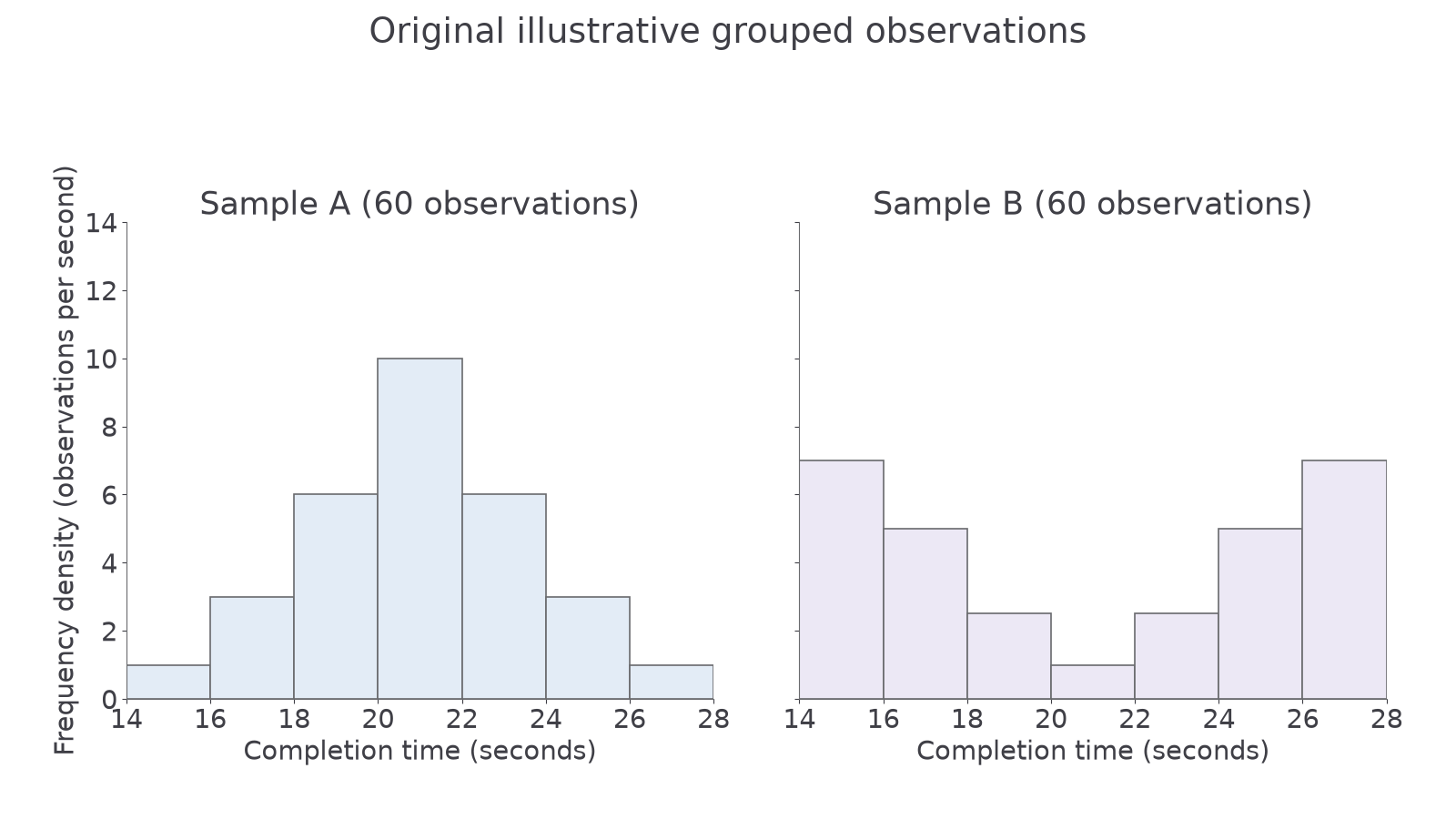
Both have $60$ observations and midpoint-based mean estimate $21\,\mathrm s$ . Symmetry makes those means equal, although A has a central mound and B has a central trough. Equal means and symmetry do not determine shape.

Check class widths before comparing bar heights: with unequal widths, area still represents frequency. A small sample or very wide classes may conceal skewness or two peaks. A long one-sided tail, a pile-up at a physical boundary or strong outliers also calls a Normal model into question.

Worked example 5: a central mound

Question. Assess $T\sim \mathrm N(21,9)$ for Sample A. Calculate the model probability of $18\leq T<24$ and compare it with the observed proportion.

Plan. Use the model's standard deviation, then compare the central area with the relevant class total.

\begin{aligned} \sigma&=\sqrt9=3 && \text{second parameter is variance} \\ \mathrm P(18\leq T<24)&=\Phi(1)-\Phi(-1) && \text{standardised limits} \\ &=0.6826894921\ldots && \text{Normal calculator} \\ \text{observed proportion}&=\frac{12+20+12}{60}=0.7333\ldots && \text{three included classes} \end{aligned}

Why this step? Comparing probabilities with proportions puts the model and sample on the same scale.

Answer. A's symmetric single mound and observed central proportion of about $0.733$ give some support to the model, whose prediction is about $0.683$ . This does not prove the population is Normal.

Check. The model boundaries are one standard deviation either side of $21$ , agreeing with the known central proportion.

Continue this lesson.

You’re previewing NovaLearn without an account. Create a free account to read the rest.

Create free account

Last Accessed

Pure Mathematics

Mechanics

Statistics

N2, N3 - Choosing and checking distribution models

Selecting a model from the process

Checking binomial mean and variance

Checking Normal models against data

Continue this lesson.

Learn faster with Nova