B11 - Functions as models | AQA A-Level Mathematics

Translate a situation into a function, fit its parameters and use its outputs with sensible inputs. You will interpret what a model assumes, compare predictions with observations, and refine a model when evidence shows that an assumption needs to change.

Variables, units and the model domain

Can two models agree with the same observation yet predict different futures? Suppose both predict $600$ visitors after $4$ days, but one eventually levels off near $1200$ and the other near $1800$ . Matching one observation is only a beginning. First we need to define what each model's variables mean.

Mathematical model

A mathematical model represents selected features of a situation using variables, relationships and simplifying assumptions. Its predictions depend on those assumptions and the circumstances in which they are reasonable. For example, a fixed fee plus a constant hourly charge gives a linear cost model; it does not account for every possible extra charge.

Define input and output units before writing an equation. Decide whether the input is a continuous measurement or an integer count, and state practical bounds. A formula can accept an input algebraically even when that input has no meaning in the situation. Coefficient units must make every added term an amount in the output unit.

You already know

A fixed amount plus a constant rate gives a line with an intercept. Direct proportionality has no fixed amount. A function's mathematical domain and range must be narrowed when context imposes further restrictions.

A cost model can predict a fee for zero work when a setup or call-out charge applies. Negative time, by contrast, need not represent any permitted service. The linear cost rule below is constructed from its assumptions; it is not in the formula booklet.

Worked example 1: a continuous input

Question. A technician charges £18 plus £12 per hour. Jobs last at most $6$ hours and fractions of an hour are charged proportionately. Define $C(h)$ in pounds, interpret its constants, and calculate the cost for $2.5$ hours.

Plan. Add the fixed fee to rate times time, then restrict the time to the stated service interval.

\begin{aligned} C(h)&=18+12h && \text{fixed fee plus time charge}\\ 0&\leq h\leq6 && \text{continuous time in hours}\\ C(2.5)&=18+12(2.5)=48 && \text{substitute the job duration} \end{aligned}

Why this step? The hourly rate has units of pounds per hour, so multiplying by hours gives pounds that can be added to the fixed fee.

Answer. $C(h)=18+12h$ , $0\leq h\leq6$ . The intercept is the £18 call-out fee; the gradient is £12 per additional hour. The predicted cost is £48.

Check. The time charge is £30, so adding £18 gives £48. A zero-hour booking would still incur the fixed fee under the stated model.

Change the kind of input next: it counts items rather than measuring time. The same fixed-plus-variable structure now needs an integer domain.

Worked example 2: a discrete input

Question. A printer charges £600 to set up a batch and £1.20 per item. A batch can contain any whole number from $0$ to $500$ items. Define $C(n)$ in pounds and find the cost for $125$ items.

Plan. Add setup and per-item costs, and list the permitted kind of input.

\begin{aligned} C(n)&=600+1.20n && \text{setup plus production}\\ n&\in\{0,1,\ldots,500\} && \text{whole-item counts}\\ C(125)&=600+1.20(125)=750 && \text{evaluate the model} \end{aligned}

Why this step? A fractional item is not a permitted batch count, even though the linear formula could be evaluated there.

Answer. $C(n)=600+1.20n$ on the stated integer set; $125$ items cost £750. The gradient represents £1.20 for each additional item.

Check. $125$ lies within the capacity, and its variable cost is £150, giving £750 including setup.

Specifying the domain is part of modelling, not an optional note added after the calculation.

Watch out

Wrong: give $0\leq n\leq500$ alone for a count model and thereby allow fractional inputs. Right: say $n$ is an integer, or list the integer set explicitly.

Use a new setup charge and capacity in the next model.

Fitting parameters and selecting a form

A model family supplies the mathematical structure; observations determine its constants. If a tank loses the same amount each minute, a linear model represents that assumption. If a quantity falls by a factor of four when a positive distance doubles, an inverse-square model may be more suitable.

Parameter

A parameter is a value held fixed within a chosen model while its input varies. In $V(t)=a-bt$ , $a$ and $b$ are parameters, while $t$ is the input. Different fitted values give different members of the same model family.

Substitute observations as equations, solve for the parameters, and check the fit. Equal input steps with constant output differences support a line. A symmetric rise and fall can support a quadratic over a bounded region; a process tending towards a ceiling can support a function with a horizontal asymptote. Data support a choice; they do not prove that its assumptions hold forever. No universal model-selection or fitting formula is supplied in the formula booklet.

Worked example 3: fit a constant outflow

Question. A tank holds $900$ litres at $t=0$ and $750$ litres after $6$ minutes. Assume no inflow and a constant outflow. Fit $V(t)=a-bt$ and find its sensible operating interval.

Plan. Use the initial amount for $a$ , determine the loss per minute, then stop the model when the tank empties.

\begin{aligned} a&=900 && \text{initial volume}\\ 750&=900-6b && \text{second observation}\\ b&=25 && \text{loss in litres per minute}\\ 900-25t&=0\quad\Longrightarrow\quad t=36 && \text{empty tank} \end{aligned}

Why this step? The line predicts negative volumes after emptying, so the contextual domain ends at its zero-volume time.

Answer. $V(t)=900-25t$ , with $V$ in litres, $t$ in minutes and $0\leq t\leq36$ . The parameter $b=25$ is the assumed constant outflow rate.

Check. $V(6)=900-150=750$ ; $V(36)=0$ . These checks confirm the fit, rather than proving the outflow assumption.

Change the assumed relationship from constant loss to inverse-square decrease. The fitting step still means substituting an observation into the chosen structure.

Worked example 4: check a proposed inverse-square form

Question. A proposed signal-strength model is $S(d)=k/d^2$ , with $d>0$ measured in metres. The strength is $12$ units at $2$ metres and $3$ units at $4$ metres. Find $k$ and check whether both observations fit.

Plan. Fit $k$ from the first pair, then predict the second strength independently.

\begin{aligned} 12&=\frac{k}{2^2} && \text{fit the first observation}\\ k&=48 && \text{multiply by }4\\ S(4)&=\frac{48}{16}=3 && \text{check the second observation} \end{aligned}

Why this step? The second observation can test the fitted relationship because it was not needed to determine its single parameter.

Answer. $S(d)=48/d^2$ , and both observations fit. The parameter has units of strength units times square metres when $d$ is measured in metres.

Check. Doubling distance divides this model's strength by four, matching the change from $12$ to $3$ . The formula is undefined at zero distance.

Two conditions can determine two parameters within a specified family. They do not identify a unique function among every possible family. Mechanism, further observations and behaviour near boundaries help decide whether the family is useful.

Watch out

Wrong: “The line matches the two given points, so the real outflow is constant.” Right: the points determine the line under that assumption; a separate observation can challenge the assumption.

Fit another inverse-square model, then compare with a second observation.

Using outputs and admissible solutions

Substituting an input predicts an output; solving an output equation finds the inputs producing a target. A model can give several valid inputs for the same target, so use its stated domain before accepting or rejecting solutions.

For a price-demand model, mean revenue is price times mean demand. If price is euros per item and demand is items per day, the product is euros per day. This contextual relationship is not in the formula booklet: learn it. A mean demand need not be a whole number, since it describes an average across days.

Worked example 5: two prices give the same revenue

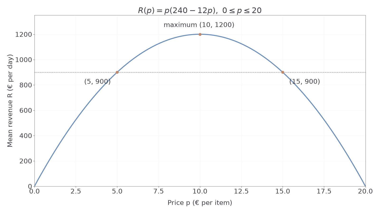
Question. Mean daily demand is modelled by $q(p)=240-12p$ items per day, where $p$ is euros per item and $0\leq p\leq20$ . Find the revenue model, its maximum, and the prices giving €900 per day.

Plan. Multiply price by demand, complete the square for the maximum, then solve the target equation.

\begin{aligned} R(p)&=p(240-12p) && \text{price times demand}\\ &=-12(p-10)^2+1200 && \text{complete the square}\\ R(p)=900&\quad\Longrightarrow\quad p^2-20p+75=0 && \text{rearrange the target}\\ (p-5)(p-15)&=0 && \text{factorise} \end{aligned}

Why this step? The completed square reveals the maximum, while factorisation finds both target prices rather than selecting only one branch.

Answer. $R(p)=240p-12p^2$ , with maximum €1200 per day at $p=10$ . Revenue €900 occurs at $p=5$ or $15$ , both within the domain.

Check. Demand is $180$ at price €5 and $60$ at price €15; both products give €900 per day.

The graph shows the two price branches. A revenue value alone does not identify a unique price without an additional branch restriction.

A quadratic mean-revenue model with its maximum and two prices giving nine hundred euros per day

Change only the revenue target next. The roots are no longer integers, so retain full precision until the final prices.

Worked example 6: a different target needs rounding

Question. Under the same demand model, find the prices giving €600 per day, to $2$ decimal places.

Plan. Solve the quadratic target equation and retain both roots in the stated domain.

\begin{aligned} 240p-12p^2&=600 && \text{set the target revenue}\\ p^2-20p+50&=0 && \text{rearrange}\\ (p-10)^2&=50 && \text{complete the square}\\ p&=10\pm5\sqrt2 && \text{take both square roots} \end{aligned}

Why this step? The two prices lie on opposite sides of the maximum and both satisfy $0\leq p\leq20$ , so neither should be rejected.

Answer. The prices are €2.93 or €17.07 per item, to $2$ decimal places.

Check. At the exact roots, $R=1200-12(50)=600$ . The rounded prices give revenues close to €600, with the small difference caused by rounding.

AQA modelling tasks may use calculator equation-solving when an exact answer is not requested. State what the solutions mean and use the precision the question asks for. The quadratic completing-square method used here is not supplied in the formula booklet.

Watch out

Wrong: reject the higher price just because demand is lower there. Revenue depends on both price and demand. Right: check each candidate against the stated domain and the target equation.

Change the target again and round only at the end.

Checking predictions and limitations

Check predictions against observations that were not merely used for fitting. A mismatch may challenge an assumption, although measurement error or natural variation can also contribute. Inspect the possible outputs and the long-term behaviour as well as a few individual predictions.

Interpolation, extrapolation and limitation

Interpolation predicts within the observed input interval; extrapolation predicts beyond it. A limitation identifies where or why a model may fail, such as a constant growth assumption becoming unreasonable as resources run out. “It is inaccurate” alone does not identify a limitation.

A contextual domain and an interval supported by observations are different. A formula may remain defined for all $t\geq0$ even when evidence supports its predictions only for a short interval. The long-term results below follow from the model's algebra; they are not formula-booklet entries.

Worked example 7: check a saturating total

Question. Cumulative visitors after $t$ days are modelled by $V(t)=1200t/(t+4)$ , $t\geq0$ . An independent observation is $1020$ visitors after $12$ days. Calculate the prediction, compare it with the observation, and state the model's long-term implication.

Plan. Evaluate at $12$ , calculate the discrepancy, and rewrite the fraction to reveal its ceiling.

\begin{aligned} V(12)&=\frac{1200(12)}{16}=900 && \text{predicted visitors}\\ 1020-900&=120 && \text{observed minus predicted}\\ V(t)&=1200-\frac{4800}{t+4} && \text{separate the limiting constant}\\ V(t)&\longrightarrow1200\quad(t\longrightarrow\infty) && \text{the fraction tends to zero} \end{aligned}

Why this step? The rewritten form shows that every finite-time prediction remains below the limiting total.

Answer. The model underpredicts the observation by $120$ visitors. Its range is $[0,1200)$ , and it approaches $1200$ visitors in the long term. A growing potential audience could make that fixed ceiling unsuitable.

Check. $V(0)=0$ , and solving $V(t)=1200$ would require $1200t=1200t+4800$ , which is impossible.

Change only the initial baseline in the next model. The same saturating increase now begins above zero and has a correspondingly higher ceiling.

Worked example 8: a nonzero baseline

Question. A visitor model is $U(t)=300+1200t/(t+4)$ , $t\geq0$ . Calculate its prediction at $12$ days, state its range, and explain whether it could reproduce an observation of $1510$ visitors at any permitted time.

Plan. Add the baseline to the previous prediction and to both bounds of the previous range.

\begin{aligned} U(12)&=300+900=1200 && \text{add the initial baseline}\\ U(t)&=1500-\frac{4800}{t+4} && \text{show the new ceiling}\\ 300&\leq U(t)<1500 && \text{nonnegative permitted time} \end{aligned}

Why this step? An observation above an upper bound for all model outputs cannot be recovered by choosing a different time.

Answer. The prediction is $1200$ , the range is $[300,1500)$ , and $1510$ is impossible within this model because it exceeds its ceiling.

Check. $U(0)=300$ ; at $t=4$ , $U(4)=900$ , between the stated bounds.

A disagreement establishes a limitation or incompatibility, rather than identifying its exact cause. A useful criticism names the assumption and its contextual consequence: for instance, a fixed audience ceiling may fail if the audience keeps expanding.

Watch out

Wrong: include a horizontal limiting total in the range automatically. Right: check whether a finite permitted input attains it; these two rational models approach their ceilings but never reach them.

Apply the same baseline-and-ceiling reasoning to a new function.

Refining assumptions and checking again

A refinement changes an assumption in response to evidence, then checks the new predictions. Changing a limiting-total parameter retains a saturating model family; removing saturation altogether changes its mathematical structure.

The original visitor model $V(t)=1200t/(t+4)$ gives $V(4)=600$ , but underpredicts the independent $12$ -day observation of $1020$ by $120$ . Suppose audience research suggests that the ceiling should be higher. Raising the ceiling alone is not enough: refit the other parameter to preserve the calibration observation, then compare predictions.

Worked example 9: increase the assumed audience

Question. Use $W(t)=1800t/(t+b)$ , $t\geq0$ , to preserve $W(4)=600$ . Find $b$ and compare the prediction at $12$ days with the observed $1020$ .

Plan. Fit $b$ using the calibration point, then calculate the error at the separate check point.

\begin{aligned} 600&=\frac{1800(4)}{4+b} && \text{preserve calibration}\\ 4+b&=12\quad\Longrightarrow\quad b=8 && \text{solve for the parameter}\\ W(12)&=\frac{21600}{20}=1080 && \text{independent prediction}\\ 1080-1020&=60 && \text{overprediction} \end{aligned}

Why this step? Checking the same observation used for fitting would only confirm the fit; the separate observation tests the changed prediction.

Answer. $W(t)=1800t/(t+8)$ . It overpredicts by $60$ , an improvement in absolute error over the original model's $120$ at this check point.

Check. $W(4)=7200/12=600$ , so the calibration remains unchanged. Both models are defined for all nonnegative times.

The curves agree at the calibration point yet approach different long-term totals, answering the opening question visually.

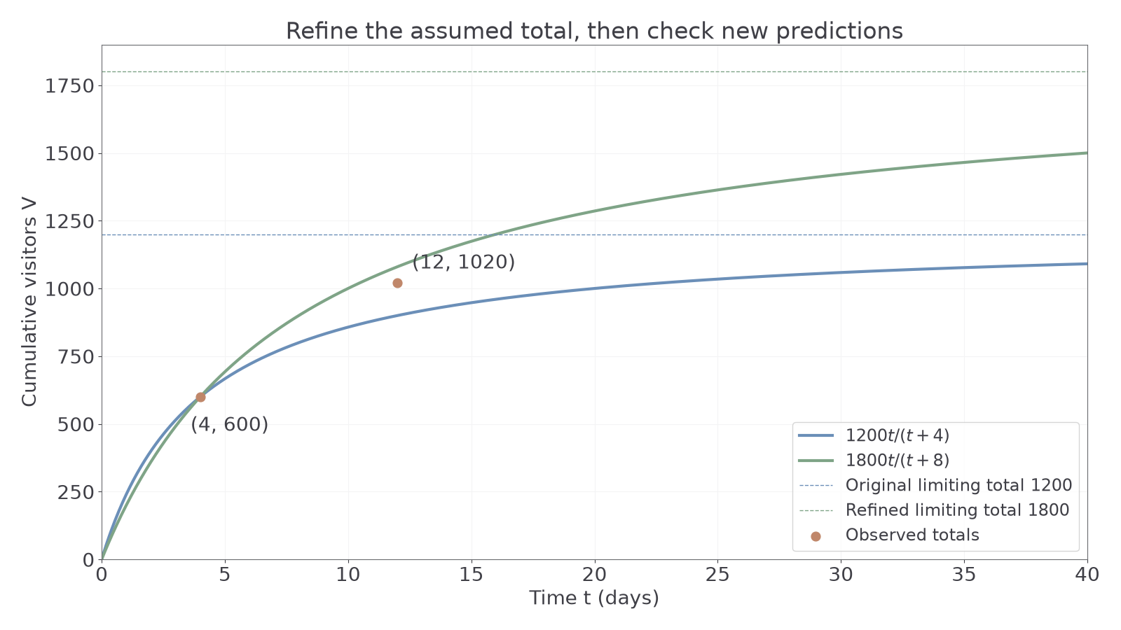
Original and refined visitor models with their distinct limiting totals and recorded check points

Change only the proposed ceiling again, from $1800$ to $2400$ , while keeping the same calibration. A larger ceiling need not give a better check-point prediction.

Worked example 10: a further change can fit less well

Question. Fit $Z(t)=2400t/(t+b)$ , $t\geq0$ , to $Z(4)=600$ . Compare its $12$ -day prediction with the observed $1020$ and the previous two models.

Plan. Refit $b$ , then compare absolute errors at the same independent input.

\begin{aligned} 600&=\frac{2400(4)}{4+b} && \text{same calibration}\\ 4+b&=16\quad\Longrightarrow\quad b=12 && \text{fit the new ceiling}\\ Z(12)&=\frac{28800}{24}=1200 && \text{new prediction}\\ |1200-1020|&=180 && \text{absolute error} \end{aligned}

Why this step? Comparing every model at the same observation makes “better” mean a specific smaller prediction error, rather than a larger parameter.

Answer. $Z(t)=2400t/(t+12)$ . Its error $180$ is larger than both the original error $120$ and the first refinement's error $60$ . This proposed change fits this check less well.

Check. $Z(4)=9600/16=600$ : even the model with the worst check-point error matches the calibration exactly.

The three models all pass through $(4,600)$ , yet their long-term predictions are $1200$ , $1800$ and $2400$ . Exact agreement at one input leaves a great deal undecided. These fitted functions are derived here and are not in the formula booklet. Further independent observations and audience evidence are needed before choosing a model for future predictions.

The modelling cycle is to specify the question and variables, state assumptions, fit a proposed relationship, use it, interpret discrepancies, then refine and check again. More parameters can improve a fit to known data without improving future predictions.

Watch out

Wrong: “The refined model matches the calibration, so it is valid for every future time.” Right: calibrate on one set of observations and test on further observations; relate any claimed improvement to the actual prediction being checked.

Fit a different ceiling while retaining the same calibration and check observation.

Quick Recap

Define variables, units, assumptions and a sensible input domain.
Fit parameters within a chosen family, then check observations not used in fitting.
Interpret outputs and retain every solution allowed by the context.
Inspect ranges and long-term behaviour, and test refinements against further evidence.

The opening models can agree at $4$ days yet approach different totals: matching a calibration observation does not determine the future.

Last Accessed

Pure Mathematics

Mechanics

Statistics

B11 - Functions as models

Variables, units and the model domain

Fitting parameters and selecting a form

Using outputs and admissible solutions

Checking predictions and limitations

Refining assumptions and checking again

Quick Recap

Learn faster with Nova