I3, I4 - Trapezium rule and numerical models | AQA A-Level Mathematics

Estimate integrals and bound areas using numerical integration (I3), then use numerical methods to find totals and threshold times in context (I4). You will distinguish a careful calculation from the reliability of the measurements and model behind it.

Ordinates and trapezia

How could five flow readings tell you how much water a pump delivers between them? Joining consecutive readings by straight lines gives trapezia whose areas estimate the total. First build that method for a curve; later you will apply it to rates.

You already know

A trapezium with parallel sides of lengths $u$ and $v$ , separated by perpendicular distance $h$ , has area $\tfrac12(u+v)h$ . This area formula is not in the formula booklet: learn it.

An ordinate is a function value $y_i=f(x_i)$ , represented by a vertical height from the horizontal axis. With $n$ equally spaced strips there are $n+1$ ordinates. For inputs $0,1,2,3,4$ , that means five ordinates but only four strips.

Adding the individual expressions $\tfrac h2(y_0+y_1)$ , $\tfrac h2(y_1+y_2)$ , and so on counts each interior ordinate twice. Each endpoint occurs only once.

Trapezium rule

For $n$ equal-width strips across $[a,b]$ , with $y_i=f(a+ih)$ ,

\int_a^b f(x)\,dx\approx \frac h2\left[(y_0+y_n)+2(y_1+\cdots+y_{n-1})\right] \qquad h=\frac{b-a}{n}

In the formula booklet.

Use the combined formula only for equal spacing. With unequal spacing, add $\tfrac12(x_{i+1}-x_i)(y_i+y_{i+1})$ separately for each strip. This separate-strip expression follows from the recalled trapezium area formula; it is not separately supplied in the booklet.

Worked example 1: five ordinates, four strips

Question. Use five ordinates to estimate $\int_0^4\sqrt{1+x}\,dx$ by the trapezium rule, to four significant figures.

Plan. Count strips, evaluate the five heights, then apply endpoint weights $1$ and interior weights $2$ .

\begin{aligned} n&=5-1=4 && \text{count the gaps} \\ h&=\frac{4-0}{4}=1 && \text{equal strip width} \\ (y_0,y_1,y_2,y_3,y_4)&=(1,\sqrt2,\sqrt3,2,\sqrt5) && \text{evaluate the heights} \\ T&=\frac12[1+\sqrt5+2(\sqrt2+\sqrt3+2)] && \text{apply the weights} \\ &=6.764298358\ldots && \text{keep calculator digits} \end{aligned}

Why this step? The five heights delimit four trapezia; dividing the interval length by five would use the wrong width.

Answer. The estimate is $6.764$ to four significant figures.

Check. The ordinates increase from $1$ to $\sqrt5$ , so an area of about $4\times1.7$ is sensible. The value is an estimate, not an exact integral.

Change only the number of strips, from four to eight. The original ordinates stay, while the new midpoints make the straight segments follow the curve more closely.

Worked example 2: refining the same integral

Question. Estimate $\int_0^4\sqrt{1+x}\,dx$ with eight equal-width strips, to four significant figures.

Plan. Use $h=0.5$ and nine ordinates; retain exact square roots until the final calculation.

\begin{aligned} h&=\frac48=0.5 && \text{new spacing} \\ y_i&=\sqrt{1+0.5i}\quad (i=0,\ldots,8) && \text{nine heights} \\ T&=\frac{0.5}{2}\left[1+\sqrt5+ 2\sum_{i=1}^{7}\sqrt{1+0.5i}\right] && \text{endpoint and interior weights} \\ &=6.781165548\ldots && \text{evaluate the weighted sum} \end{aligned}

Why this step? Doubling the strips adds real function evaluations. It does not mean doubling the old estimate or merely halving its error.

Answer. The refined estimate is $6.781$ to four significant figures.

Check. Exact integration gives $\tfrac23(5\sqrt5-1)=6.786893258\ldots$ , so this refinement is closer than the four-strip result. The power-integration method used for that check is not in the formula booklet: learn it.

For unequal inputs $0,1,3$ with ordinates $2,3,5$ , the widths are $1$ and $2$ . Adding their separate trapezia gives $\tfrac12(1)(2+3)+\tfrac12(2)(3+5)=10.5$ ; there is no common width for the combined formula.

Watch out

Wrong: “Five ordinates on $[0,4]$ give $h=4/5$ .” Ordinates are heights; strips are the gaps between them. Correct: $n=4$ and $h=4/4=1$ . Double only the interior heights.

For the check, change the function but retain the eight-strip calculation and the distinction between heights and gaps.

Curvature and area bounds

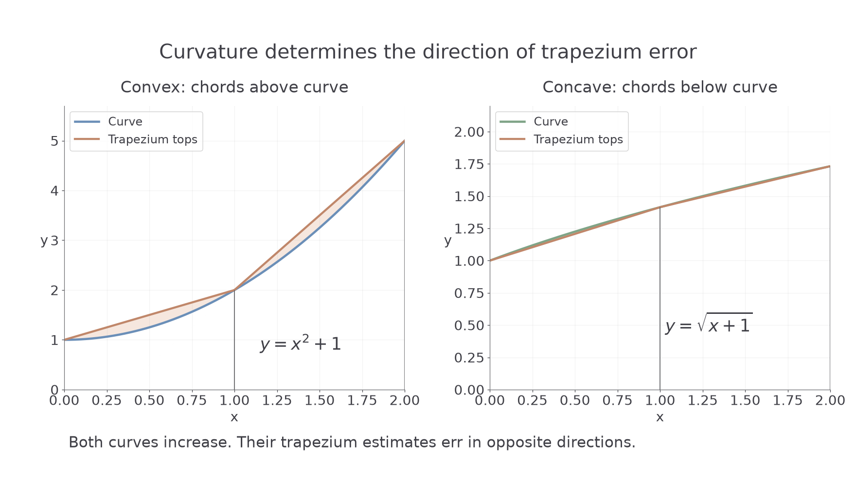
Whether a trapezium overestimates depends on the curve's bending, not simply on whether the curve rises or falls.

For a convex curve, bending upwards with $f''(x)>0$ , its chords lie above the curve; trapezia overestimate the integral. For a concave curve, bending downwards with $f''(x)<0$ , chords lie below the curve; trapezia underestimate. The same statements with non-strict curvature give non-strict bounds. These curvature and chord tests are not in the formula booklet: learn them.

Two increasing curves with opposite curvature show trapezium tops above a convex curve and below a concave curve

For a continuous increasing function, left-end rectangles give a lower bound and right-end rectangles an upper bound. For a decreasing function their roles reverse. With equal-width strips, the trapezium estimate is the mean of the left and right rectangle sums, $T=(L+U)/2$ , because it averages each strip's two endpoint heights. These rectangle bounds and this mean relationship are not separately supplied in the formula booklet: derive them from the heights. Combining monotonicity with curvature can improve a bound.

Worked example 3: bounds for a concave curve

Question. Use unit-width rectangles to bound $I=\int_0^4\sqrt{1+x}\,dx$ , then improve one bound using trapezia.

Plan. Use increasing heights for rectangle bounds, then use concavity to place the trapezium estimate.

\begin{aligned} L&=1+\sqrt2+\sqrt3+2=6.146264369\ldots && \text{left heights} \\ U&=\sqrt2+\sqrt3+2+\sqrt5=7.382332347\ldots && \text{right heights} \\ f''(x)&=-\frac1{4(1+x)^{3/2}}<0 && \text{concave throughout} \\ T&=\frac{L+U}{2}=6.764298358\ldots && \text{trapezium estimate} \end{aligned}

Why this step? Concavity places each chord below the curve, so $T$ is a lower bound, stronger than the smaller left-rectangle sum.

Answer. $T<I<U$ , with $T=6.764298358\ldots$ and $U=7.382332347\ldots$ .

Check. The exact value $6.786893258\ldots$ is above $T$ and below $U$ , as required.

Change only the function to $1+x^2$ , keeping the interval and unit-width strips. Both functions increase, but this one bends upwards, reversing which bound the trapezium improves.

Worked example 4: bounds for a convex curve

Question. Use unit-width rectangles and trapezia to bound $J=\int_0^4(1+x^2)\,dx$ .

Plan. Find the rectangle bounds, then use the positive second derivative to locate $T$ .

\begin{aligned} L&=1+2+5+10=18 && \text{left rectangles} \\ U&=2+5+10+17=34 && \text{right rectangles} \\ T&=\frac12[1+17+2(2+5+10)]=26 && \text{trapezia} \\ f''(x)&=2>0 && \text{convex throughout} \end{aligned}

Why this step? The chords lie above this curve, so $T$ improves the upper bound, even though the curve is increasing just like the previous one.

Answer. $18<J<26$ , a tighter interval than $18<J<34$ .

Check. Exact integration gives $J=4+64/3=76/3$ , which lies between $18$ and $26$ .

For a curve with one sign of curvature, subdividing existing strips makes the trapezium estimate move towards the integral: downwards for convex curves and upwards for concave curves. If curvature changes sign, different strips may err in opposite directions; a table of values alone usually does not establish what happens between its entries.

An integral is signed. A particle whose velocity changes linearly through $2,0,-2\,\mathrm{m\,s^{-1}}$ at $0,2,4\,\mathrm{s}$ has zero displacement, but travels $4\,\mathrm m$ : the positive and negative signed trapezia cancel, while their magnitudes add. The zero and straight segments are known here. Taking absolute sample values is not a general shortcut for total area when a crossing could be hidden between them. The signed-integral and total-area distinction is not in the formula booklet: learn it.

Watch out

Wrong: “The function is increasing, so trapezia overestimate.” Increasing describes the first derivative, not chord position. Correct: check curvature; for $5-e^{-x}$ , $f'>0$ but $f''<0$ , so trapezia underestimate its integral.

The next check changes the function again. Decide which bound is improved from curvature, not from the increasing ordinates.

Continue this lesson.

You’re previewing NovaLearn without an account. Create a free account to read the rest.

Create free account

Last Accessed

Pure Mathematics

Mechanics

Statistics

I3, I4 - Trapezium rule and numerical models

Ordinates and trapezia

Curvature and area bounds

Continue this lesson.

Learn faster with Nova