B7 - Function graphs and intersections | AQA A-Level Mathematics

An equation tells you much more than a collection of plotted points. You will sketch polynomial, modulus and reciprocal graphs, use their intersections to solve equations and inequalities, and recognise proportional relationships on suitable axes.

Polynomial shapes and intercepts

How can one cubic curve pass through the same height three times? Start with $y=(x+2)(x-1)^2$ : it crosses the horizontal axis once, touches it once, and bends between them. Its equation tells you which features a sketch must show.

You already know

A product is zero when at least one factor is zero. Substituting $x=0$ gives the point where a graph meets the vertical axis, provided zero is allowed.

A sketch shows the important shape and labelled features without requiring a table of equally spaced points. For $y=mx+c$ , the gradient is $m$ and the vertical intercept is $c$ . The line $y=c$ is horizontal; $x=c$ is vertical. A vertical line is not a function of $x$ , since its one input has many outputs.

Axis intercept

An axis intercept is a point where a graph meets an axis. For $y=f(x)$ , solve $f(x)=0$ for the horizontal intercepts, and calculate $f(0)$ for the vertical intercept. For example, $y=2x-6$ has intercepts $(3,0)$ and $(0,-6)$ .

The highest power controls a polynomial's ends. A positive quadratic rises at both ends; a negative quadratic falls at both ends. A positive cubic falls to the left and rises to the right; a negative cubic reverses that behaviour. Cubics can have three distinct real roots, a repeated root and another root, or only one real root. For example, $x^3+x=x(x^2+1)$ has only the real root zero. The graph of $x^3$ crosses at its triple root without turning there.

At a simple or triple root the sign changes, so the graph crosses the axis. At a double root it keeps the same sign and touches the axis. These sketching rules and intercept results are not in the formula booklet: learn them.

Worked example 1: a cubic with a double root

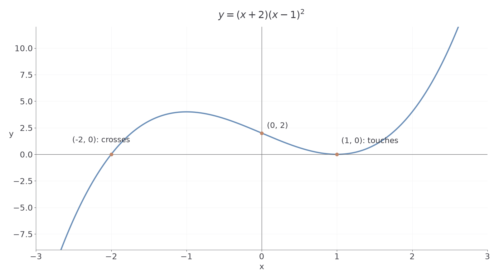
Question. Sketch $y=(x+2)(x-1)^2$ , labelling its axis intercepts.

Plan. Find the roots and their multiplicities, calculate the vertical intercept, then use the leading term for the ends.

\begin{aligned} (x+2)(x-1)^2&=0 && \text{horizontal intercepts}\\ x&=-2\text{ or }1 && \text{one simple, one double root}\\ y(0)&=2(-1)^2=2 && \text{vertical intercept}\\ (x+2)(x-1)^2&=x^3-3x+2 && \text{positive cubic term} \end{aligned}

Why this step? The squared factor cannot change sign at $x=1$ , so the curve touches there rather than crossing.

Answer. Draw a smooth cubic crossing at $(-2,0)$ , touching at $(1,0)$ , and passing through $(0,2)$ . Its left end falls and its right end rises.

Check. At $x=-3$ the output is $-16$ ; at $x=2$ it is $4$ , consistent with the two ends.

The labelled picture makes the different root behaviours visible. Exact turning-point coordinates are not needed for this sketch.

A cubic crossing at minus two, touching at one and meeting the vertical axis at two

Now change only the overall sign. The roots remain in place, but every nonzero height changes sign.

Worked example 2: reverse the leading sign

Question. Sketch $y=-(x+2)(x-1)^2$ , labelling its axis intercepts.

Plan. Retain the roots and multiplicities, then reverse the heights and end behaviour.

\begin{aligned} y&=0\quad\Longrightarrow\quad x=-2\text{ or }1 && \text{same zero factors}\\ y(0)&=-2 && \text{include the leading minus}\\ y&=-x^3+3x-2 && \text{negative leading term} \end{aligned}

Why this step? Multiplying by $-1$ changes the signs on both sides of each root together, so a crossing remains a crossing and a touch remains a touch.

Answer. The curve crosses at $(-2,0)$ , touches at $(1,0)$ , and passes through $(0,-2)$ . Its left end rises and its right end falls.

Check. At $x=2$ , the output is $-4$ , the negative of the first curve's output.

Factorisation determines the roots; a rough drawing must agree with it.

Watch out

Wrong: “Every root is a crossing.” A squared factor gives a touch. Right: use the factor's multiplicity and the sign on either side, rather than joining the intercepts with a guessed wave.

Try a cubic with three simple roots instead of a double root.

The modulus of a linear expression

Modulus measures distance from zero: $|-4|=4$ and $|4|=4$ . On a graph, it lifts negative outputs above the horizontal axis.

Modulus

For a real number $u$ ,

|u|=\begin{cases}u&u\geq0\\-u&u<0\end{cases}

For example, $|-3|=3$ . It is never $-3$ . Not in the formula booklet: learn it.

To sketch $y=|ax+b|$ , first consider the line $y=ax+b$ . Keep its nonnegative section and reflect its negative section in the horizontal axis. For $a\ne0$ , the vertex occurs where $ax+b=0$ . A constant outside the modulus moves every height afterwards: $|2x-4|+1$ is different from $|2x-3|$ .

Worked example 3: form the two straight pieces

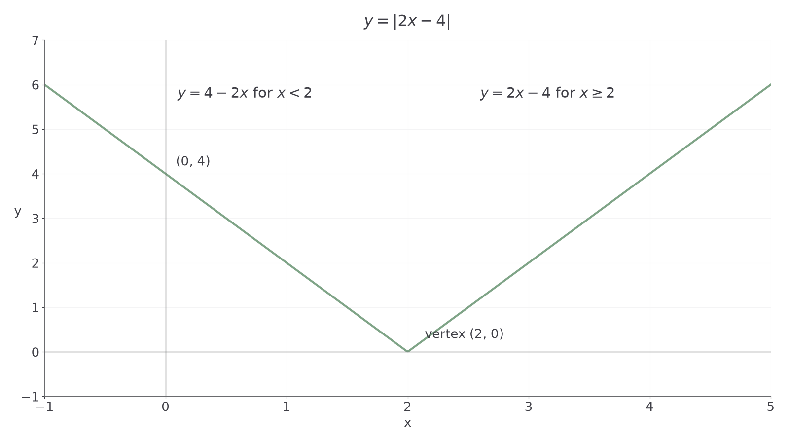
Question. Sketch $y=|2x-4|$ and write its two linear pieces.

Plan. Find where the expression inside changes sign, then apply the modulus definition on each side.

\begin{aligned} 2x-4&=0\quad\Longrightarrow\quad x=2 && \text{change of sign}\\ |2x-4|&=\begin{cases}4-2x&x<2\\2x-4&x\geq2\end{cases} && \text{reverse negative outputs}\\ y(0)&=4 && \text{vertical intercept} \end{aligned}

Why this step? On $x<2$ , the entire expression is negated: $-(2x-4)=4-2x$ .

Answer. Draw a V with vertex $(2,0)$ , vertical intercept $(0,4)$ , and gradients $-2$ and $2$ on its left and right arms.

Check. At $x=1$ , the definition and the left piece both give $2$ ; both pieces give zero at $x=2$ .

The corner is where the two formulae agree, so there is no break in the curve.

The two linear pieces of a modulus graph joining at the vertex two zero

The next example adds only a vertical shift. It preserves the two gradients but changes the intercepts and the lowest output.

Worked example 4: add a constant outside

Question. Sketch $y=|2x-4|-3$ , giving the vertex and all axis intercepts.

Plan. Move the previous V down by $3$ , then solve for its zero heights.

\begin{aligned} \text{vertex}&=(2,-3) && \text{subtract }3\text{ from its height}\\ y(0)&=4-3=1 && \text{vertical intercept}\\ |2x-4|&=3 && \text{horizontal intercepts}\\ 2x-4&=3\text{ or }-3 && \text{two distances from zero}\\ x&=\frac72\text{ or }\frac12 && \text{solve each line} \end{aligned}

Why this step? The outside subtraction occurs after the modulus, so the graph can now have negative heights.

Answer. The upward V has vertex $(2,-3)$ , intercepts $(\frac12,0)$ , $(\frac72,0)$ and $(0,1)$ , and outputs $y\geq-3$ .

Check. At either stated root the modulus is $3$ , giving zero after subtraction.

An outside multiplier also acts after the modulus. For example, $2|x|-1$ has vertex $(0,-1)$ ; $-2|x|+1$ opens downwards with vertex $(0,1)$ . These results follow from the definition and are not supplied in the formula booklet.

Watch out

Wrong: $|2x-4|=2x+4$ for all $x$ . Negate the whole expression only on its negative branch. Right: $4-2x$ for $x<2$ , and $2x-4$ for $x\geq2$ .

Change the horizontal position of the corner in the next question.

Modulus equations and inequalities

An intersection with a modulus graph must belong to the straight piece used to find it. Solving two linear equations without checking their input regions can introduce false answers.

For $|u|=c$ , a positive $c$ gives $u=c$ or $u=-c$ ; zero gives $u=0$ ; a negative $c$ gives no solutions. If the other side depends on $x$ , it too must be nonnegative at an intersection. These rules are consequences of the modulus definition, not formula-booklet entries.

Worked example 5: a V meets a sloping line

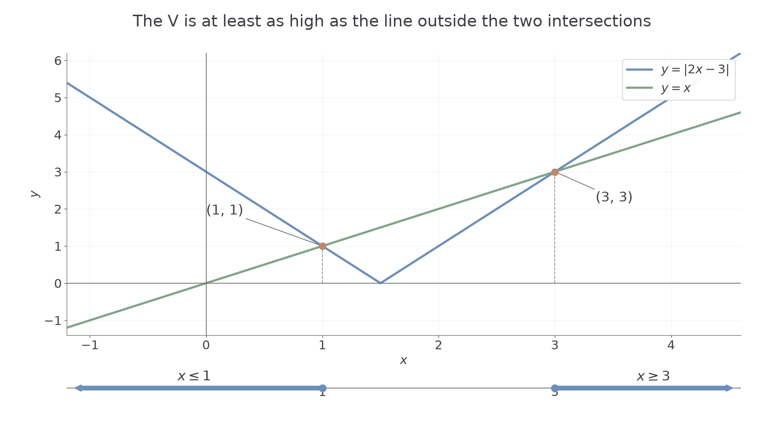
Question. Find the intersections of $y=|2x-3|$ and $y=x$ .

Plan. Split at $x=\frac32$ , solve each straight-piece equation, then check its branch.

\begin{aligned} x<\frac32:\quad 3-2x&=x && \text{left arm}\\ x&=1 && 1<\frac32\\ x\geq\frac32:\quad 2x-3&=x && \text{right arm}\\ x&=3 && 3\geq\frac32 \end{aligned}

Why this step? Each replacement of the modulus has a condition; a root obtained outside that condition would not solve the original equation.

Answer. The intersections are $(1,1)$ and $(3,3)$ .

Check. $|2(1)-3|=1$ and $|2(3)-3|=3$ , so both original equations agree.

Change only equality to an inequality. The same intersection inputs divide the regions where the V is above or below the line.

Worked example 6: which graph is higher?

Question. Solve $|2x-3|\geq x$ .

Plan. Solve on each modulus branch and retain only inputs belonging to that branch.

\begin{aligned} x<\frac32:\quad 3-2x&\geq x && \text{left arm}\\ x&\leq1 && \text{already in this branch}\\ x\geq\frac32:\quad 2x-3&\geq x && \text{right arm}\\ x&\geq3 && \text{already in this branch} \end{aligned}

Why this step? An inequality asks for whole intervals of inputs, including intersections when the sign is $\geq$ .

Answer. $x\leq1$ or $x\geq3$ , equivalently $( -\infty,1]\cup[3,\infty)$ .

Check. At $x=0$ , $3\geq0$ is true; at $x=2$ , $1\geq2$ is false; at $x=4$ , $5\geq4$ is true.

Graphically, the V lies below the line between the two intersections. Thus $|2x-3|<x$ instead gives $1<x<3$ . Strict inequalities exclude the intersection inputs. AQA may ask you to use intersections “Hence, or otherwise”; state the intervals, not just the boundary roots.

The graphs of y equals the modulus of two x minus three and y equals x intersect at one one and three three; the modulus is at least as large on x at most one or x at least three

Watch out

Wrong: square both sides of $|2x-3|\geq x$ for every real $x$ without checking signs. If $x<0$ , the original inequality is automatically true, while squaring may change it. Branches preserve the original meaning directly.

The next V has its corner further right. Give a complete set of intervals.

Reciprocal graphs and asymptotes

For $y=6/x$ , inputs $1,2,3$ give outputs $6,3,2$ . Larger positive inputs give smaller positive heights, but no permitted input gives zero.

Asymptote

An asymptote is a straight line approached by a curve in a specified limiting direction. A vertical asymptote $x=c$ has outputs tending to positive or negative infinity on at least one side as $x$ approaches $c$ . A horizontal asymptote $y=d$ describes heights as $x$ tends to positive or negative infinity.

For both $y=a/x$ and $y=a/x^2$ , with $a\ne0$ , zero is excluded and the axes $x=0$ , $y=0$ are asymptotes. When $a>0$ , the reciprocal $y=a/x$ has branches in quadrants I and III; when $a<0$ , they lie in quadrants II and IV. Draw asymptotes with dashed lines. Infinity describes unbounded behaviour; it is not an input you can substitute. These graph results are not in the formula booklet: learn them.

Worked example 7: a negative reciprocal

Question. Describe and sketch $y=-6/x$ , giving its asymptotes and two points.

Plan. Determine signs on either side of zero and calculate one point on each branch.

\begin{aligned} x=-2&\quad\Longrightarrow\quad y=3 && \text{negative input}\\ x=2&\quad\Longrightarrow\quad y=-3 && \text{positive input}\\ \frac{-6}{-x}&=-\frac{-6}{x} && \text{opposite inputs, opposite outputs} \end{aligned}

Why this step? The denominator's sign changes across zero, so the branches lie on opposite sides of the horizontal axis.

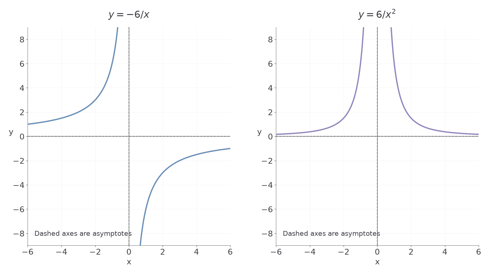
Answer. Draw branches in quadrants II and IV through $(-2,3)$ , $(2,-3)$ , approaching dashed $x=0$ and $y=0$ . There are no axis intercepts; the graph has rotational symmetry about the origin.

Check. At $x=100$ , $y=-0.06$ , close to zero; at $x=0.01$ , $y=-600$ , far below the axis.

The next example changes only the denominator's power. Squaring removes its sign, changing the symmetry and the branch positions.

Worked example 8: square the denominator

Question. Describe and sketch $y=-6/x^2$ , giving its asymptotes and two points.

Plan. Use $x^2>0$ for nonzero inputs, then calculate equal and opposite inputs.

\begin{aligned} x=-2&\quad\Longrightarrow\quad y=-\frac64=-\frac32 && \text{left branch}\\ x=2&\quad\Longrightarrow\quad y=-\frac64=-\frac32 && \text{right branch}\\ \frac{-6}{(-x)^2}&=\frac{-6}{x^2} && \text{equal heights} \end{aligned}

Why this step? Every denominator is positive, so both branches have the numerator's negative sign.

Answer. Both branches lie below the axis, are symmetric in the vertical axis, and approach dashed $x=0$ , $y=0$ . They pass through $(\pm2,-\frac32)$ and have no axis intercepts.

Check. At $x=\pm1$ both heights are $-6$ ; increasing $|x|$ to $10$ gives $-0.06$ , nearer zero.

A positive numerator puts both reciprocal-square branches above the axis. The following comparison shows that case beside the negative reciprocal.

A negative reciprocal with opposite branches and a positive reciprocal-square with two upper branches

A shifted form $y=d+a/(x-c)$ has vertical asymptote $x=c$ and horizontal asymptote $y=d$ . Its outputs exclude $d$ , since a nonzero numerator divided by a finite denominator cannot be zero. For example, $2+3/(x-1)$ has asymptotes $x=1$ , $y=2$ , and all real outputs except $2$ . A negative reciprocal-square graph instead attains every negative output: solving $y=-a/x^2$ , with $a>0$ and $y<0$ , gives the real nonzero inputs $x=\pm\sqrt{-a/y}$ . These results are not in the formula booklet. More general graphs can cross a horizontal asymptote; an asymptote describes limiting behaviour, not a universal barrier.

Watch out

Wrong: put a point at $(0,0)$ to join reciprocal branches. The function is undefined at zero and its heights become unbounded nearby. Draw separate branches and dashed asymptotes.

Change the negative numerator in the reciprocal-square example and use the same sketch features.

Equations as graph intersections

Graphs intersect when the same input gives the same output in both rules. Solving $f(x)=g(x)$ finds the horizontal coordinates; substituting back finds the heights.

For example, $y=x^2$ and $y=4$ meet at $(-2,4)$ and $(2,4)$ , so $x^2=4$ has two solutions. A graph usually estimates a root, while algebra can establish an exact result and show that no roots were missed. Equivalently, solve $f(x)-g(x)=0$ . This intersection rule is not in the formula booklet: learn it.

Worked example 9: a cubic meets a horizontal line

Question. Find all intersections of $y=x^3-3x+2$ and $y=2$ .

Plan. Equate heights, factor the resulting cubic, then use the line for each height.

\begin{aligned} x^3-3x+2&=2 && \text{same height}\\ x(x^2-3)&=0 && \text{factorise}\\ x&=0,\ -\sqrt3,\ \sqrt3 && \text{zero-product rule}\\ y&=2 && \text{on the horizontal line} \end{aligned}

Why this step? Removing the common height leaves a factored equation whose factors account for every solution.

Answer. The points are $(0,2)$ , $(-\sqrt3,2)$ , $(\sqrt3,2)$ .

Check. For $x=\pm\sqrt3$ , $x^3=3x$ , so the cubic's height is indeed $2$ .

Here is the answer to the opening puzzle: the same cubic reaches height $2$ at three different inputs, although it has only two distinct horizontal intercepts. Roots and intersections with another horizontal line need not have the same count.

Change only the line's gradient in the next example.

Worked example 10: a sloping line

Question. Find all intersections of $y=x^3-3x+2$ and $y=6x+2$ .

Plan. Equate heights and factor, then calculate each height using the simpler line.

\begin{aligned} x^3-3x+2&=6x+2 && \text{equate outputs}\\ x(x^2-9)&=0 && \text{collect and factor}\\ x&=-3,0,3 && \text{three roots}\\ y&=-16,2,20 && \text{substitute into }6x+2 \end{aligned}

Why this step? The roots are only inputs; the question asks for coordinate pairs, so the heights are still needed.

Answer. $(-3,-16)$ , $(0,2)$ and $(3,20)$ .

Check. At $x=-3$ , the cubic gives $-27+9+2=-16$ , matching the line.

A tangency can give one distinct intersection even if its equation has a repeated root. Count distinct points, and do not assume that a limited plotting window contains every intersection.

Watch out

Wrong: report $x=-3,0,3$ as the coordinates of the intersections. Right: pair each input with its height, unless the question asks only for the input values.

Change the gradient again and find the exact points.

Proportional relationships and graph axes

A fixed multiplier is the defining feature of proportionality. If $y=2x^2$ , doubling $x$ multiplies $y$ by four, so $y$ is proportional to $x^2$ , rather than to $x$ .

Proportional relationships

y\propto x^n\quad\Longleftrightarrow\quad y=kx^n

y\propto\frac1{x^n}\quad\Longleftrightarrow\quad y=\frac{k}{x^n}

The constant $k$ does not vary with $x$ ; use only inputs making the expression defined. Not in the formula booklet: learn it.

A graph of $y$ against the quantity to which it is proportional is a straight line through the origin, with gradient $k$ . Thus plot against $x^2$ for square proportionality or against $1/x^2$ for inverse-square proportionality. On ordinary axes, only direct proportionality to $x$ gives that straight-line test. On transformed axes, the origin may represent a limit rather than an attainable original input.

Worked example 11: an inverse-square relationship

Question. $y$ is inversely proportional to $x^2$ for $x>0$ . Given $y=9$ when $x=2$ , find its equation and the output at $x=6$ . State axes giving a straight line.

Plan. Substitute the observation into $y=k/x^2$ , then use the fitted constant.

\begin{aligned} 9&=\frac{k}{2^2} && \text{use the observation}\\ k&=36 && \text{multiply by }4\\ y(6)&=\frac{36}{6^2}=1 && \text{predict the new output} \end{aligned}

Why this step? The same $k$ must work at every permitted input; it is not a second variable.

Answer. $y=36/x^2$ , giving $y=1$ at $x=6$ . Plot $y$ against $1/x^2$ for a line through the origin with gradient $36$ .

Check. The input triples, so its square increases by nine and the output falls from $9$ to $1$ .

Change only the proportionality to the direct square relationship. The fitting method remains substitution, but the scaling reverses.

Worked example 12: a square relationship

Question. $y$ is proportional to $x^2$ . Given $y=18$ when $x=3$ , find its equation and the output at $x=5$ . State axes giving a straight line.

Plan. Use $y=kx^2$ , find $k$ , then evaluate the new input.

\begin{aligned} 18&=k(3^2) && \text{fit the constant}\\ k&=2 && \text{divide by }9\\ y(5)&=2(5^2)=50 && \text{use the model} \end{aligned}

Why this step? The multiplier relates $y$ to $x^2$ , so the graph must use $x^2$ as its horizontal variable.

Answer. $y=2x^2$ , giving $50$ . Plot $y$ against $x^2$ for a line through the origin with gradient $2$ .

Check. At $x=-3$ , the same equation gives $18$ : equal squares give equal heights.

A line with a nonzero vertical intercept adds a fixed amount and is not direct proportionality to its horizontal variable.

Watch out

Wrong: “A straight graph proves $y\propto x$ .” Right: check both that it passes through the origin and that the horizontal variable really is $x$ , rather than $x^2$ or $1/x^2$ .

Use a new observation to fit another square relationship.

Quick Recap

Use roots, multiplicities, the vertical intercept and end behaviour to sketch polynomials.
Split a linear modulus at its zero; keep branch restrictions when solving equations and inequalities.
Reciprocal graphs have excluded inputs and dashed asymptotes; denominator powers determine their symmetry.
Equate heights for intersections and choose the correct horizontal variable for proportionality.

The opening cubic reaches height $2$ three times: at $x=-\sqrt3$ , $0$ and $\sqrt3$ .

Last Accessed

Pure Mathematics

Mechanics

Statistics

B7 - Function graphs and intersections

Polynomial shapes and intercepts

The modulus of a linear expression

Modulus equations and inequalities

Reciprocal graphs and asymptotes

Equations as graph intersections

Proportional relationships and graph axes

Quick Recap

Learn faster with Nova