F6 - Linearising exponential and power data | AQA A-Level Mathematics

Choose logarithmic axes that turn a power or exponential model into a straight line. Use its gradient and intercept to estimate the original constants, then check the model against data and the range of any prediction.

Power-law logarithmic axes

The outputs $2,8,32,128$ occur at inputs $1,2,4,8$ . Can a straight line reveal the relationship hiding in these curved data?

Doubling $x$ multiplies $y$ by $4$ , suggesting $y=2x^2$ . Logging both coordinates turns that repeated multiplication into equal additions. Throughout, take logs of numerical measurements expressed in fixed stated units; do not mix units within a table.

You already know

A line $Y=mX+c$ has gradient $m=\Delta Y/\Delta X$ and intercept $c=Y-mX$ . Also, $\log_{10}(ax^n)=\log_{10}a+n\log_{10}x$ for $a,x>0$ . These results are not in the formula booklet: learn them.

For $y=ax^n$ , set $X=\log_{10}x$ , $Y=\log_{10}y$ . Both $x$ and $y$ must be positive. A log–log plot puts the transformed output against the transformed input.

Straightening a power law

For $a>0$ and $x>0$ ,

\begin{aligned} y=ax^n&\quad\Longrightarrow\quad Y=nX+c \\ X&=\log_{10}x\qquad Y=\log_{10}y\qquad c=\log_{10}a \\ n&=\text{gradient}\qquad a=10^c \end{aligned}

If both logs are natural, $c=\ln a$ and $a=e^c$ , while the gradient is still $n$ .

Not in the formula booklet: learn it.

On ordinary paper, calculate the logs and space their values uniformly. Logarithmic graph paper instead spaces the original labels by their logarithms. Either way, the horizontal mathematical coordinate is $\log x$ , not $x$ .

Worked example 1: recovering the opening model

Question. Use a log–log line to identify $y=ax^n$ for the following exact data.

$x$	$1$	$2$	$4$	$8$
$y$	$2$	$8$	$32$	$128$
$X=\log_{10}x$ , 4 d.p.	$0$	$0.3010$	$0.6021$	$0.9031$
$Y=\log_{10}y$ , 4 d.p.	$0.3010$	$0.9031$	$1.5051$	$2.1072$

Plan. Use well-separated transformed points for the gradient and the point with $X=0$ for the intercept.

\begin{aligned} n&=\frac{\log_{10}128-\log_{10}2}{\log_{10}8-\log_{10}1}=2 && \text{gradient using unrounded logs} \\ c&=\log_{10}2 && X=0\text{ at }x=1 \\ a&=10^{\log_{10}2}=2 && \text{undo the logarithm} \end{aligned}

Why this step? The intercept is the logarithm of the multiplier, so it needs back transformation before it can be used as $a$ .

Answer. $y=2x^2$ .

Check. At $x=4$ , $2(4^2)=32$ ; the model also gives the other three entries.

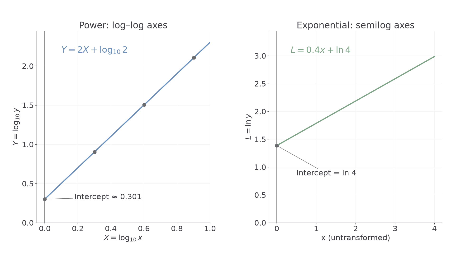
Power data become a straight line on log–log axes, while exponential data use an untransformed horizontal axis

The left panel is the opening dataset. Now change only the power from $2$ to $-2$ , keeping the multiplier $2$ . The transformed line's gradient reverses; its intercept stays fixed.

Worked example 2: a negative power

Question. A log–log fitted line passes through $(X,Y)=(0,\log_{10}2)$ and $(1,\log_{10}2-2)$ . Find $a,n$ in $y=ax^n$ and predict $y$ at $x=4$ .

Plan. Calculate the line's gradient, undo its intercept, then use the original model.

\begin{aligned} n&=\frac{(\log_{10}2-2)-\log_{10}2}{1-0}=-2 && \text{gradient} \\ a&=10^{\log_{10}2}=2 && \text{back transform intercept} \\ y(4)&=2(4^{-2})=1/8 && \text{original variables} \end{aligned}

Why this step? The negative gradient is the exponent $n$ , not a negative multiplier; the original outputs remain positive.

Answer. $y=2x^{-2}$ , and $y=1/8$ at $x=4$ .

Check. At $X=1$ , $x=10$ and the model gives $y=0.02$ ; $\log_{10}(0.02)=\log_{10}2-2$ , the stated line point.

Changing units can move a log–log line without changing its gradient. In the opening model, replace $x$ by $u=10x$ . Then $y=2(u/10)^2=0.02u^2$ : the exponent remains $2$ , while the multiplier changes from $2$ to $0.02$ . This follows from the unsupplied power-law transformation above, and is why a fitted exponent can survive a change of length units.

Watch out

Wrong: “The intercept is $0.3010$ , so $a=0.3010$ .” The intercept is $\log_{10}a$ , so $a=10^{0.3010}\approx2$ . Only the gradient is read directly as a parameter of the power model.

Try another fitted line, changing the line data while keeping the same axes and recovery method.

Exponential semilogarithmic axes

An exponential model needs only its output logged: the original input already appears as the coefficient of a logarithm.

For example, $y=4e^{0.4x}$ gives $\ln y=\ln4+0.4x$ , a straight line in $x$ . Logging $x$ as well would spoil that linear relationship.

Straightening an exponential model

For $y=kb^x$ , with $k,b>0$ ,

\begin{aligned} L=\ln y&=mx+c\qquad m=\ln b\qquad c=\ln k \\ b&=e^m\qquad k=e^c\qquad y=e^ce^{mx} \end{aligned}

With $\log_{10}y$ instead, $m=\log_{10}b$ , $c=\log_{10}k$ , so $b=10^m$ and $k=10^c$ .

Not in the formula booklet: learn it.

A semilog plot uses $x$ horizontally and $\ln y$ vertically. It requires $y>0$ ; $x$ may be zero or negative. A positive gradient gives $b>1$ , a negative gradient gives $0<b<1$ , and zero gradient gives the constant model $y=k$ . These interpretation rules follow from the back transformation and are not supplied separately.

Worked example 3: a positive logged gradient

Question. A fitted line is $\ln y=0.4x+\ln4$ . Find $k,b$ in $y=kb^x$ , then predict $y$ at $x=3$ to three significant figures.

Plan. Exponentiate the intercept and gradient separately, and use their unrounded values for the prediction.

\begin{aligned} k&=e^{\ln4}=4 && \text{intercept gives }\ln k \\ b&=e^{0.4}\approx1.49 && \text{gradient gives }\ln b \\ y(3)&=4e^{0.4(3)}=4e^{1.2}\approx13.3 && \text{use unrounded parameter} \end{aligned}

Why this step? The slope is $0.4=\ln b$ , not $b$ . A base $0.4$ would describe decay, contradicting the positive slope.

Answer. $k=4$ , $b=e^{0.4}\approx1.49$ , and the prediction is $y\approx13.3$ .

Check. At $x=0$ , $y=4$ ; increasing $x$ by $1$ multiplies the model output by $e^{0.4}>1$ .

The right panel of the earlier diagram shows that line. Change only its gradient to $-0.4$ . The original multiplier stays $4$ , but the exponential base becomes its reciprocal.

Continue this lesson.

You’re previewing NovaLearn without an account. Create a free account to read the rest.

Create free account

Last Accessed

Pure Mathematics

Mechanics

Statistics

F6 - Linearising exponential and power data

Power-law logarithmic axes

Exponential semilogarithmic axes

Continue this lesson.

Learn faster with Nova