L1 - Data displays and histograms | AQA A-Level Mathematics

Read a display by asking what its positions, heights and areas represent. You will interpret histograms, boxplots and cumulative frequency graphs, compare distributions and turn recorded frequencies into proportions.

Choosing a display for one variable

Can the tallest histogram bar contain fewer cars than a shorter bar? It can: a narrow interval may have a high concentration of cars but a smaller total count. Choosing the display and reading its scale come before comparing its shapes.

You already know

A frequency counts observations. A proportion is a count divided by the total count. A rectangle's area is width multiplied by height.

A car's make is a category; its mass is a numerical measurement. The AQA workbook's fuel-type numbers are category codes, so the difference between two codes is not a measured difference in fuel. ReferenceNumber is an identifier, not a numerical characteristic to average.

Single-variable data

Single-variable data record one characteristic for each observation. A bar chart uses separate bars for categories; a histogram groups a numerical variable into intervals whose widths have meaning.

Match a display to the question you want to answer. This is a choice of information, not a rule that one display is always best.

Question	Useful display	Information it exposes
Which car make occurs most often?	Bar chart	Counts for separate categories
Where are masses concentrated?	Histogram	Shape, intervals and tails
Which service has shorter, more consistent waits?	Boxplots on one scale	Median and quartile spread
How many journeys take at most a stated time?	Cumulative frequency graph	Count up to a threshold

The current AQA car workbook has $3827$ selected records: BMW $551$ , FORD $1089$ , TOYOTA $275$ , VAUXHALL $1069$ and VOLKSWAGEN $843$ . These counts add to the workbook total. They describe its restricted selection of makes, registration weeks and keeper regions, rather than national market shares. The workbook is a $2017$ Department for Transport database extract, containing selected cars from $2002$ and $2016$ .

A boxplot can hide two clusters with similar quartiles. A histogram shows more shape, but changing its class boundaries can change that appearance. A long tail towards high values indicates positive skew; a long tail towards low values indicates negative skew. Look towards the tail rather than the tallest bar. These shape descriptions are not in the formula booklet: learn them. Read labels, units, class boundaries, key and total count before interpreting either. An unfamiliar display is manageable once you identify what one point or symbol represents.

Key idea

Choose a display using the variable type and the question; then identify the group and scale that its values actually describe.

A categorical code can look numerical while still being only a label. Use that distinction here.

Histogram density and area

A histogram spreads each class frequency over its interval, so height measures concentration and area measures count.

These illustrative waiting-time classes contain a total of $80$ waits. The last column gives the heights of their histogram bars.

Waiting time $t$ in minutes	Frequency	Width	Frequency density
$0\le t<5$	$10$	$5$	$2$
$5\le t<10$	$20$	$5$	$4$
$10\le t<20$	$30$	$10$	$3$
$20\le t<40$	$20$	$20$	$1$

The tallest bar contains $20$ waits, while the lower but wider next bar contains $30$ .

Frequency density

\text{frequency density}=\frac{\text{frequency}}{\text{class width}} \qquad \text{frequency}=\text{class width}\times\text{frequency density}

Use the actual measurement boundaries. For $10\le t<20$ , the width is $20-10=10$ .
Not in the formula booklet: learn it.

For measurements rounded to whole units, a printed class such as $15$ – $24$ may instead have boundaries $14.5$ and $24.5$ . Use the stated recording convention. With true density on the axis, rectangle area equals frequency; with an axis merely proportional to density, first determine its common scale factor from a known class. For example, if an area of $6$ grid squares represents $18$ observations, each square represents $18/6=3$ . An area of $10$ such squares then represents $30$ observations. These are area units, rather than vertical-axis readings.

Worked example 1: read a whole class

Question. Using the waiting-time class data above, find the frequency in $10\le t<20$ and the proportion of all $80$ waits in that class.

Plan. Multiply width by height, then divide the class count by the total.

\begin{aligned} f&=(20-10)\times3=30 && \text{area is frequency}\\ \text{proportion}&=\frac{30}{80}=\frac38 && \text{class count over total} \end{aligned}

Why this step? Height $3$ alone describes waits per minute of interval, not the number of waits.

Answer. There are $30$ waits, giving proportion $3/8$ .

Check. The four areas sum to $10+20+30+20=80$ .

Now change only the requested interval: its upper boundary lies inside the same class. The raw observations' positions are unknown, so the resulting count is an estimate.

Worked example 2: use part of a bar

Question. Use those class data to estimate how many of the $80$ waits satisfy $10\le t<16$ , and their proportion. State the assumption.

Plan. Use the area over the shorter interval, assuming a uniform spread within its class.

\begin{aligned} \widehat f&=(16-10)\times3=18 && \text{partial rectangle area}\\ \text{estimated proportion}&=\frac{18}{80}=0.225 && \text{divide by all waits} \end{aligned}

Why this step? The constant bar height allocates the same estimated count to each minute of the class; the original grouped data do not prove that allocation.

Answer. An estimated $18$ waits, proportion $0.225$ , assuming observations are uniformly distributed within $[10,20)$ .

Check. The interval covers $6/10$ of the class width, and $(6/10)\times30=18$ .

The authentic AQA mass histogram below excludes the $92$ impossible zero masses, leaving $3735$ positive masses. Mass is recorded in $\mathrm{kg}$ , including $75\,\mathrm{kg}$ for an average driver. Its class frequencies are $92,1020,1768,770,85$ , with the boundaries shown.

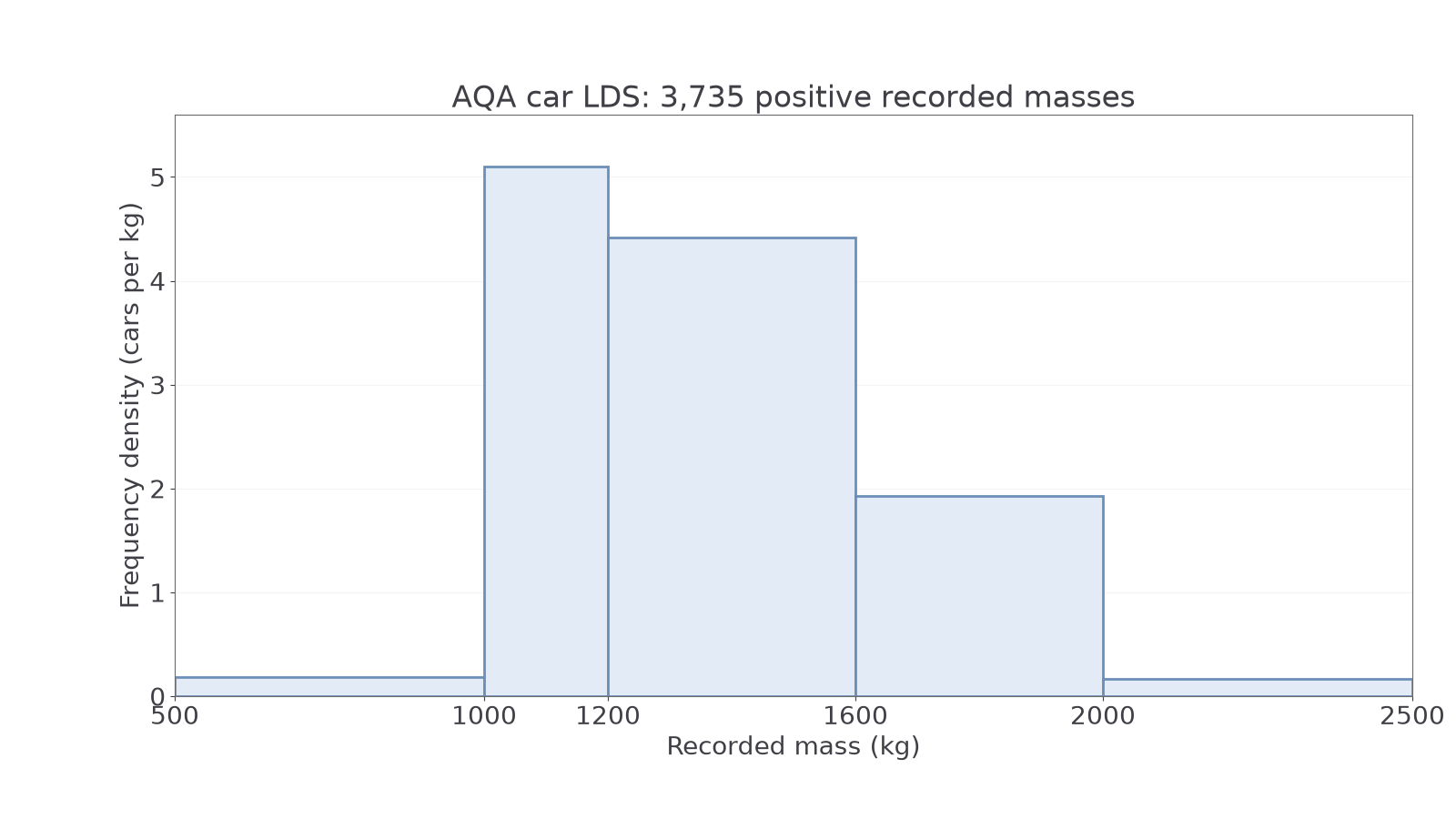
Histogram of 3735 positive AQA car masses, with unequal class widths and frequency density in cars per kg

The $1200$ – $1600\,\mathrm{kg}$ bar has height $1768/400=4.42$ cars per $\mathrm{kg}$ . The $1000$ – $1200\,\mathrm{kg}$ bar is taller, at $1020/200=5.1$ , but contains fewer cars. That answers the opening question with real data.

Source: AQA car LDS, $2017$ DfT Stock Vehicle Database; public sector information under Open Government Licence v3.0. The exclusion applies to this mass analysis.

Watch out

Wrong: “The bar of height $5.1$ contains more cars than the bar of height $4.42$ .” Unequal widths make heights incomparable as counts. Right: compare areas $200\times5.1=1020$ and $400\times4.42=1768$ .

For the next partial-bar estimate, identify both the interval width and the total number of observations from the question itself.

Continue this lesson.

You’re previewing NovaLearn without an account. Create a free account to read the rest.

Create free account

Last Accessed

Pure Mathematics

Mechanics

Statistics

L1 - Data displays and histograms

Choosing a display for one variable

Histogram density and area

Continue this lesson.

Learn faster with Nova