L2 - Scatter diagrams, regression and correlation | AQA A-Level Mathematics

Interpret paired observations, supplied correlation coefficients and the coefficients of a given regression line. You will recognise distinct groups, keep the units and pairings intact, and distinguish an association from evidence of a causal effect.

Reading paired scatter data

Can every group show a downward association while the combined data show an upward one? Yes: differences between the groups can conceal their internal patterns. Before investigating that reversal, learn to read one paired point accurately.

You already know

A point $(x,y)$ keeps its two coordinates together. A straight line's gradient describes change in the vertical variable per unit change in the horizontal variable. A category such as fuel type can distinguish groups of points.

Bivariate data pair two measurements from the same object, person or occasion. Separately sorting the columns would invent new pairs. On a scatter diagram, check the variable and unit on each axis, then look for direction, shape, clusters and isolated points.

An upward pattern suggests positive association; a downward pattern suggests negative association. Closeness to a straight line concerns strength of linear association, not steepness. A curved pattern may be strong without being linear. An isolated point may be a possible outlier to investigate rather than delete.

These authentic AQA observations are the first six distinct EngineSize/NOX pairs encountered for each of Petrol and Diesel in the workbook. This is a deliberately selected teaching subset, not a random sample. NOX records oxides of nitrogen emissions.

ReferenceNumber	Fuel	EngineSize $(\mathrm{cm}^3)$	NOX $(\mathrm{g\,km^{-1}})$
$440$	Petrol	$1598$	$0.026$
$1465$	Petrol	$1398$	$0.010$
$3434$	Petrol	$1395$	$0.033$
$1801$	Petrol	$1598$	$0.012$
$264$	Petrol	$1998$	$0.040$
$1846$	Petrol	$1398$	$0.008$
$2330$	Diesel	$1995$	$0.023$
$2216$	Diesel	$1499$	$0.074$
$2971$	Diesel	$2967$	$0.039$
$2419$	Diesel	$1598$	$0.047$
$3809$	Diesel	$1997$	$0.059$
$1929$	Diesel	$1968$	$0.063$

Twelve authentic AQA EngineSize and NOX pairs, with different symbols for petrol and diesel

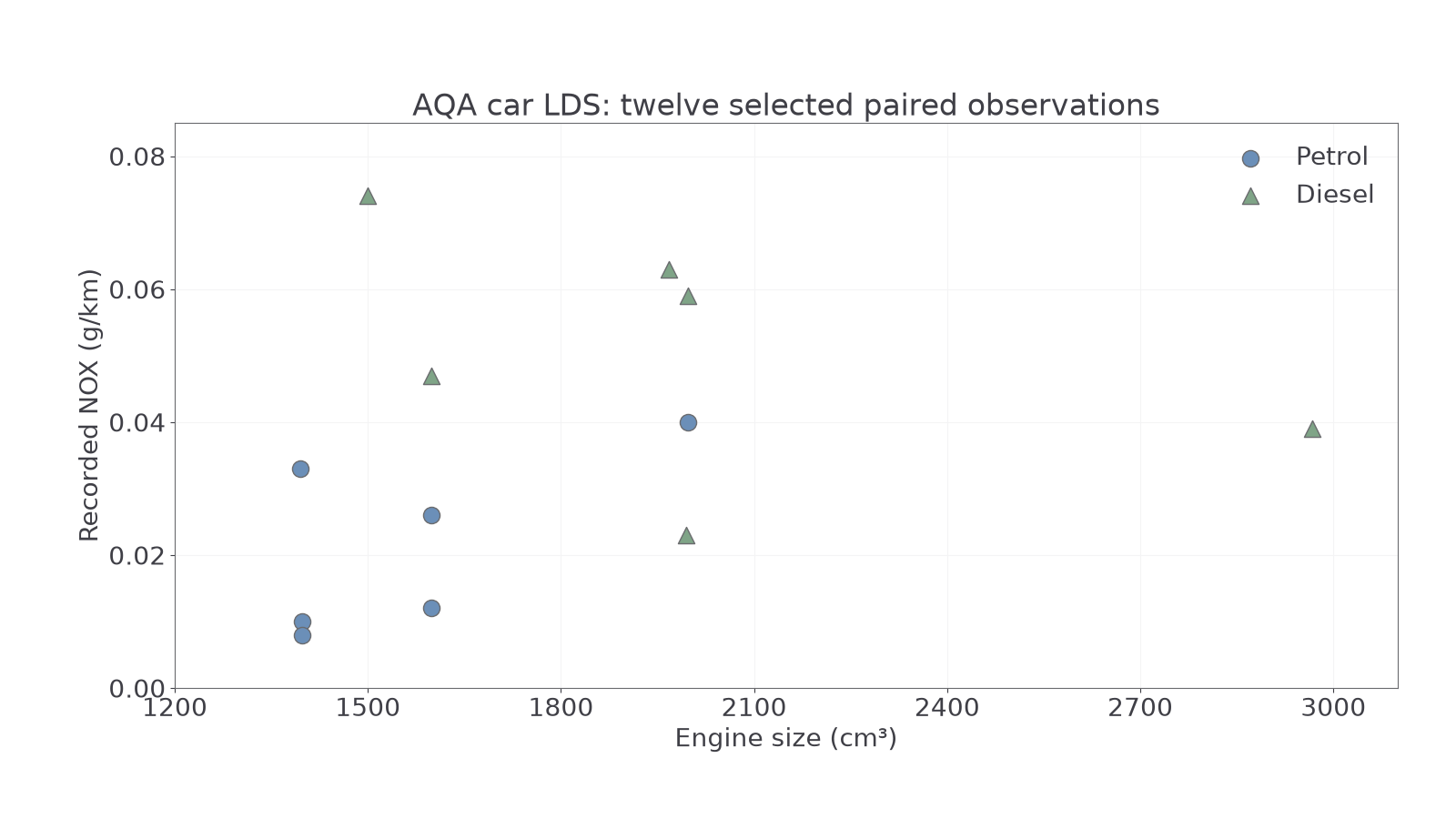
Source: AQA car LDS, $2017$ DfT Stock Vehicle Database, Open Government Licence v3.0. Decimal emissions are shown at their recorded decimal precision.

Worked example 1: locate the highest point

Question. Identify the fuel and engine size of the selected car with highest NOX.

Plan. Find the greatest vertical value, then read the same point's horizontal value and group.

\begin{aligned} \max(\mathrm{NOX})&=0.074 && \text{record }2216\\ \text{EngineSize}&=1499\,\mathrm{cm}^3 && \text{same row and point} \end{aligned}

Why this step? The highest point need not be the furthest right; the coordinates measure different quantities.

Answer. Diesel, with engine size $1499\,\mathrm{cm}^3$ .

Check. The high diesel triangle lies near $1500$ on the horizontal scale, not near $3000$ .

Change only which coordinate is extreme: find the rightmost point rather than the highest. The pairing rule stays the same.

Worked example 2: locate the rightmost point

Question. Identify the fuel and NOX of the selected car with largest engine size.

Plan. Find the greatest EngineSize, then keep its other fields attached.

\begin{aligned} \max(\text{EngineSize})&=2967\,\mathrm{cm}^3 && \text{record }2971\\ \mathrm{NOX}&=0.039\,\mathrm{g\,km^{-1}} && \text{same observation} \end{aligned}

Why this step? Pairing the largest engine with the largest NOX would create a car not present in the selected data.

Answer. Diesel, with NOX $0.039\,\mathrm{g\,km^{-1}}$ .

Check. The rightmost triangle is just below the horizontal $0.04$ gridline.

Several diesel points are above petrol points, but the groups overlap: diesel record $2330$ 's $0.023$ is below petrol record $264$ 's $0.040$ . Thus “every selected diesel has more NOX than every selected petrol” is false. The plot also does not isolate engine size as a cause, because fuel and other vehicle features vary together.

Watch out

Wrong: pair $2967$ with $0.074$ because both are column maxima. They belong to different records. Right: keep both measurements and any group label from the same row.

Exact table entries take precedence over small reading differences on a graph. You are interpreting the display, rather than being asked to construct it.

Interpreting a given correlation coefficient

A supplied correlation coefficient compresses linear direction and strength into one number; it does not report a gradient or a causal effect.

The sample product moment correlation coefficient is denoted $r$ . The sign gives direction, and its distance from zero helps compare strength of linear association. Values close to $1$ or $-1$ represent strong positive or negative linear association respectively; $r=0$ means no linear correlation, rather than no possible relationship.

Range of a correlation coefficient

-1\le r\le1

Not in the formula booklet: learn it.

A supplied value $1.08$ is impossible. A value inside the range is possible, but that alone does not verify its calculation. Words such as strong, moderate and weak are useful comparisons rather than universal numerical cutoffs; do not try to read an exact coefficient by eye from a cloud.

Worked example 3: separate sign and strength

Question. Two illustrative investigations relate study time to task-completion time. Supplied coefficients are A: $r=-0.82$ , B: $r=0.35$ . Compare direction and linear strength.

Plan. Read each sign for direction, then compare absolute magnitudes.

|-0.82|=0.82>0.35=|0.35|

Why this step? The negative sign reverses direction; it does not make the association weaker.

Answer. A has a stronger linear association and a negative direction: more study tends to accompany shorter completion time. B has a weaker positive linear association: more study tends to accompany longer completion time.

Check. A is closer to $-1$ than B is to $1$ .

Change only A's sign to positive. Its magnitude stays the same, so the strength comparison should survive.

Worked example 4: reverse direction only

Question. For the same defined variables, supplied coefficients are now A: $r=0.82$ , B: $r=0.35$ . Compare their direction and linear strength.

Plan. Repeat the sign and magnitude readings separately.

|0.82|=0.82>0.35=|0.35|

Why this step? Changing the sign of one coefficient changes direction while preserving its magnitude.

Answer. Both associations are positive: larger study times tend to accompany longer completion times. A has the stronger linear association.

Check. Both values are in $[-1,1]$ ; neither is a percentage of observations or a rate of change.

For a useful boundary case, the symmetric pairs $(-2,4),(-1,1),(0,0),(1,1),(2,4)$ lie exactly on $y=x^2$ , yet have $r=0$ . Opposite horizontal positions balance in the linear summary while the curve remains clear. A scatter diagram therefore supplies information a coefficient can hide. You are given coefficients here; their calculation is not required.

Watch out

Wrong: “ $-0.82<0.35$ , so A has weaker correlation.” That compares signed values rather than linear strength. Right: compare magnitudes, then describe each sign separately.

Use a new pair of supplied coefficients, and keep both the comparison and its context explicit.

Continue this lesson.

You’re previewing NovaLearn without an account. Create a free account to read the rest.

Create free account

Last Accessed

Pure Mathematics

Mechanics

Statistics

L2 - Scatter diagrams, regression and correlation

Reading paired scatter data

Interpreting a given correlation coefficient

Continue this lesson.

Learn faster with Nova