O3 - Normal mean hypothesis tests

The distribution of a sample mean

Individual packet masses have standard deviation $4\,\mathrm g$. How can a mean of just $16$ packets have standard deviation only $1\,\mathrm g$, and why would halving that uncertainty again require $64$ packets?

An individual packet can be unusually heavy or light. In an average, some positive and negative departures offset one another. The mean varies between samples, but less than individual observations vary within the population.

Use $\bar X$ for the random sample mean before observing the sample, and $\bar x$ for the realised mean. They are different: one has a probability distribution; the other is the number calculated from the observations.

The supplied standardisation tells us that $\bar X\sim\mathrm N(\mu,\sigma^2/n)$, with standard deviation $\sigma/\sqrt n$. This equivalent distribution is recovered from the booklet result; it is not a separate printed formula. Its variance is $\sigma^2/n$, not its standard deviation.

To see the scaling, independent observations give a sum with variance $n\sigma^2$. Dividing that sum by $n$ divides its variance by $n^2$, leaving $\sigma^2/n$. These variance-scaling facts explain the supplied formula; they are not printed separately in the booklet. Four times the sample size divides the variance by four and the standard deviation by two. Because the population is Normal, the mean's Normal distribution is exact even for a small sample under the independence assumption.

Example 2 changes only the sample size, from $16$ to $64$. The same mass interval now contains a larger proportion of sample means.

Use the known, given or assumed population variance in this method. A sample variance $s^2$ estimates population spread; it does not make that spread known. A test with unknown population variance requires another method, outside this lesson.

When a calculator asks for standard deviation, enter $\sigma/\sqrt n$, not the variance $\sigma^2/n$.

Population hypotheses and standardisation

The null specifies the population mean used to calculate the reference distribution. The observed sample mean then tells us how far the evidence departs from that claim.

Define $\mu$ in the context. For reference value $\mu_0$, use $H_0:\mu=\mu_0$. A decrease uses $H_1:\mu<\mu_0$, an increase uses $H_1:\mu>\mu_0$, and a change uses $H_1:\mu\ne\mu_0$. These hypothesis conventions are not in the formula booklet: learn them. Choose the direction before observing the sample.

Under $H_0$, replace $\mu$ by $\mu_0$ in the booklet's sampling-distribution formula. Its observed standardised value is

This is the supplied standardisation evaluated at the observed mean. It counts how many sample-mean standard deviations the result lies above or below the null mean. It is not a difference measured in individual-observation standard deviations.

Write $\Phi(z)=\mathrm P(Z\le z)$ for the standard Normal cumulative probability. A lower-tail alternative uses p-value $\Phi(z)$; an upper-tail alternative uses $1-\Phi(z)$. These tail choices are not printed in the formula booklet: learn them. A negative $z$ does not support an increase: its upper-tail p-value exceeds $0.5$.

Example 4 changes only the observed sample mean. Keep the population variance and sampling model unchanged.

AQA expects the population mean and its tested direction in the conclusion. “The batteries have changed” does not identify the quantity tested.

The next question isolates hypothesis choice so that the required tail is clear before calculation begins.

Critical values and two-tailed tests

A critical region gives a decision boundary before the sample is observed. For a continuous Normal distribution, you can allocate the significance probability exactly, assuming the model holds.

Use inverse Normal on your calculator. An upper $5\%$ tail leaves cumulative probability $0.95$ below its boundary, giving $\Phi^{-1}(0.95)=1.64485\ldots$. A lower $5\%$ tail uses $\Phi^{-1}(0.05)=-1.64485\ldots$. For a two-tailed $5\%$ test, allocate $0.025$ to each tail:

These critical values are not printed in the formula booklet; obtain them using inverse Normal rather than memorising rounded boundaries. The booklet supplies the sampling standardisation used to convert them into sample means.

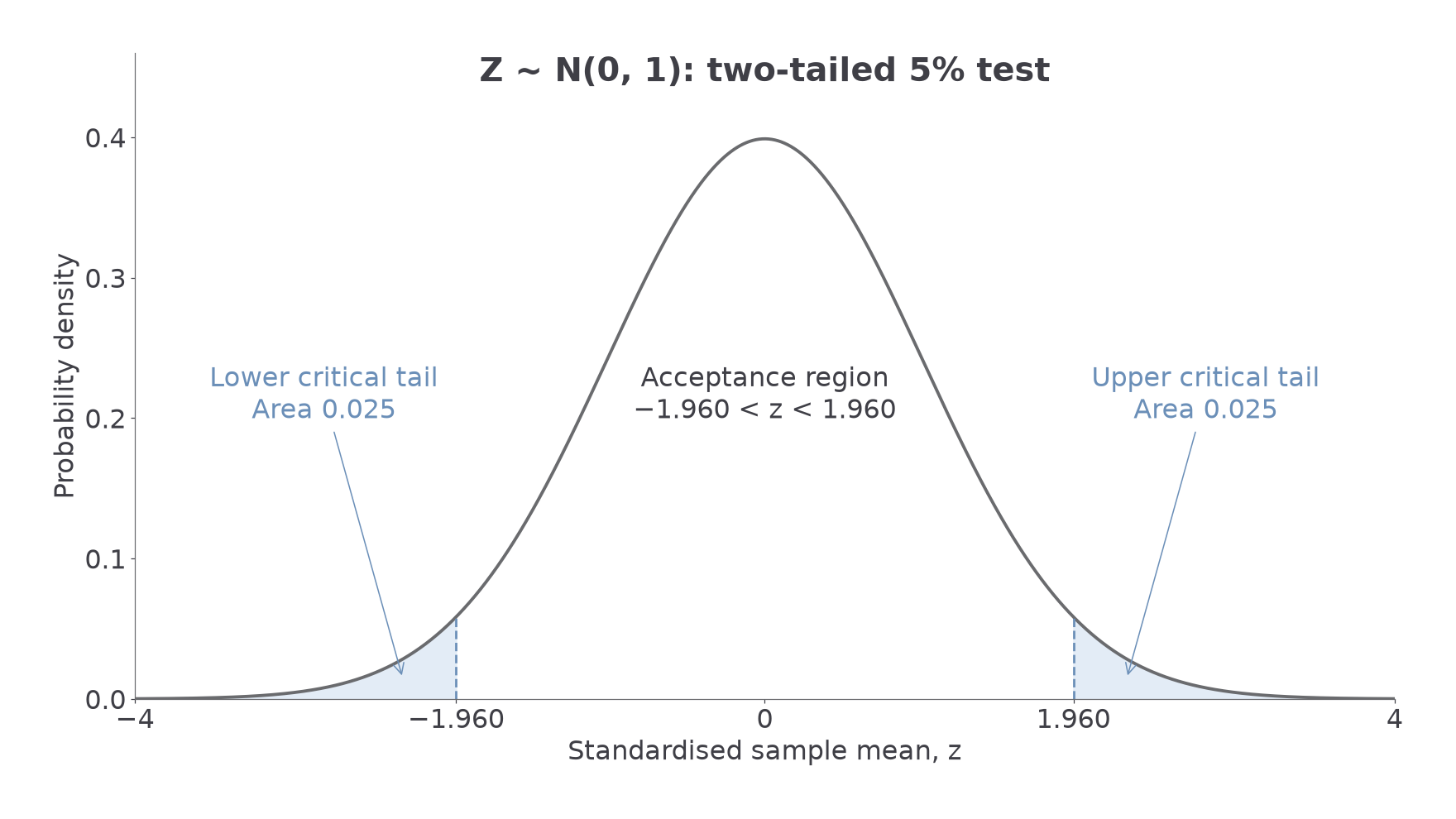
Reject when $z$ lies in either shaded tail. For a continuous variable, strict or inclusive boundary inequalities give the same probability because a single exact value has probability zero.