RP12 - Species distribution and environmental factors
Does a plant really thin out with distance from a path? Investigate how a named environmental factor is associated with one species' distribution: pair field measurements, choose an analysis and state what the evidence can establish. This lesson supports Required Practical 12; completing its written work does not demonstrate fieldwork or practical competence.
Field question and abundance measures
A precise question names the species, the factor, the habitat and how you will measure abundance.
Distribution describes where organisms occur; abundance describes how much or how many occur. Recording abundance at known positions shows distribution, so a useful question fixes all four choices: “Is soil moisture associated with the percentage cover of a named grass species in this meadow?”
Before collecting data, identify the species with a reliable key and set a sampling boundary and a rule for objects on quadrat edges. The area must include possible absences as well as dense patches. Sampling only where the species is visible biases the estimated distribution and cuts off part of the factor's range.
The factor is measured, not set
RP12 asks about the effect of a factor, but in an observational field study you measure the moisture or light already there. The factor is often called the independent variable, even though nobody manipulates it. Other factors can change along with it, so the data show an association, not a cause.
Record the unit and what the instrument actually measures: a moisture probe might report volumetric water content as a percentage, and a light meter records illuminance in lux. Distance from a path is a proxy for possible trampling, not a direct measurement of trampling intensity. Soil pH, moisture and shade might also change with distance.
Three measures of abundance
You met these in 3.7.4. Choose the one that fits the organism:
| Measure | What you record | Use it when |
|---|---|---|
| Density | Rooted individuals per quadrat | Individuals can be distinguished |
| Percentage cover | Percentage of the quadrat area the species occupies | Grasses or creeping plants overlap |
| Frequency | Percentage of quadrats in which the species occurs | Presence or absence is enough |
A species present in 12 of 20 quadrats has a frequency of 60%, however many individuals occupy each quadrat. Frequency describes a group of quadrats, so don't treat it as a continuous abundance reading from each one.
Quadrats, transects and paired data
The question decides the design: random quadrats across an area, or a belt transect along a gradient.
Random quadrats for a whole area
Use these for an association across a site:
- Map the site with two perpendicular tapes, so any position has coordinates.
- Generate coordinates in advance from a random number generator or table, so every position has the same chance of selection and you cannot favour spots by eye.
- Place the same quadrat corner at each coordinate, with the same quadrat size and edge rule throughout, so samples are comparable.
- Sample many independently selected locations, based on a pilot survey and the available area, so the sample represents variation across the site. In June 2024, a specific sample size had to be 10 or more to earn the mark.
Belt transects for a gradient
For a gradient, such as distance from a footpath, random positions could leave some stages unsampled, so use a transect:
- Lay a tape perpendicular to the path, so it runs along the gradient.
- Place quadrats at fixed intervals to make an interrupted belt transect, so stages are sampled evenly along the whole gradient. Record the interval and quadrat area.
- Repeat transects at independently chosen positions along the path, because a single line may happen to cross an unusual patch.
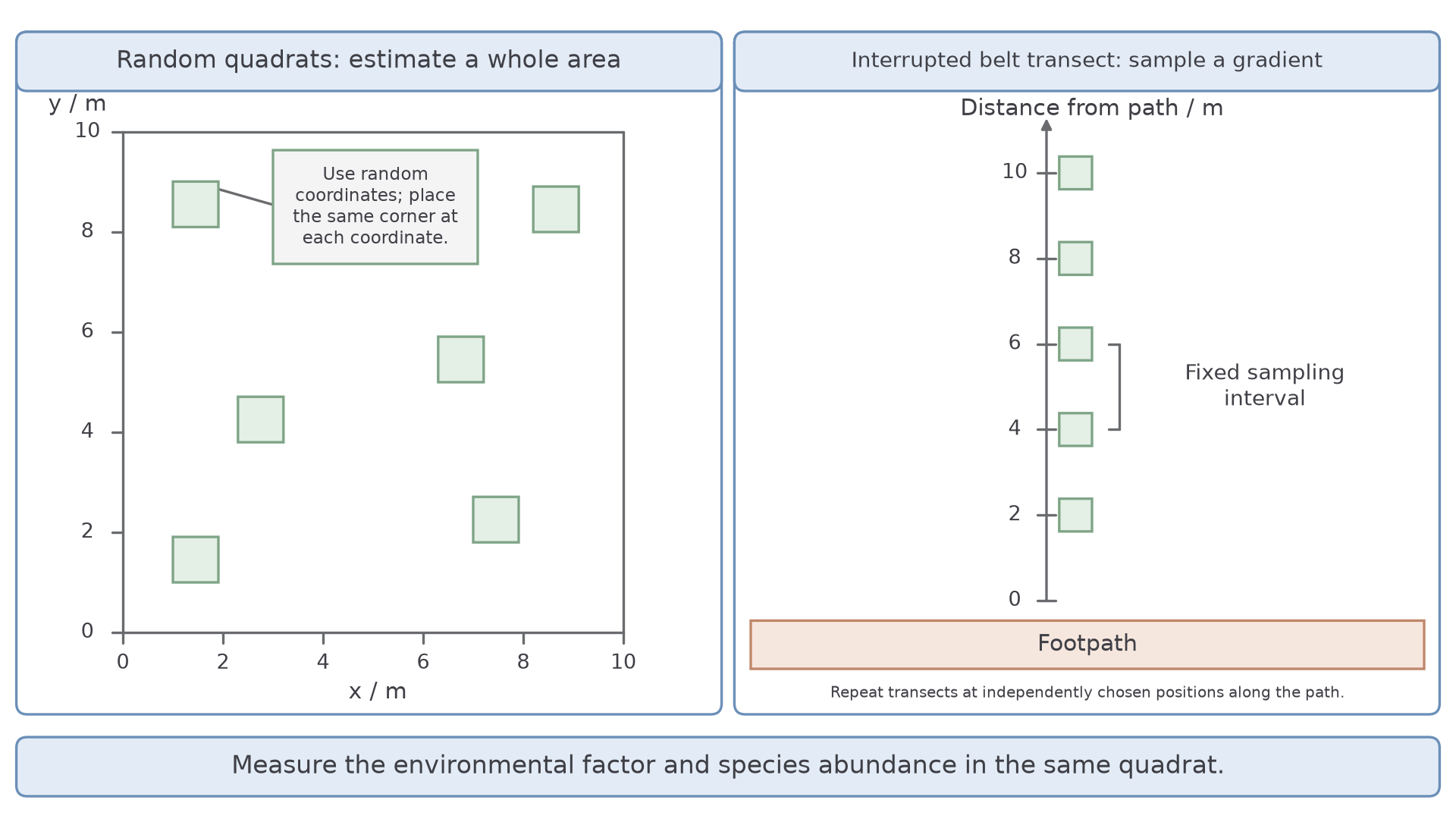
Many adjacent quadrats on one line are not equivalent to independent replicate transects. In the diagram, the left panel shows random quadrats across a 10 m by 10 m site, and the right panel shows one transect with a quadrat every 2 m.
[DIAGRAM: asset_name: quadrat-and-transect-sampling; asset_slug: quadrat-and-transect-sampling; recommended_method: retained_png; caption: Random quadrats sample a defined area, repeated interrupted belt transects sample distribution along a measured gradient.; description: Random quadrats sample a defined area; repeated interrupted belt transects sample distribution along a measured gradient.]
Pairing abundance with the factor
At each quadrat, measure both species abundance and the environmental factor, so the observations are paired. Match the instrument to the factor:
| Factor | Instrument | Keep consistent |
|---|---|---|
| Soil moisture | Calibrated probe | Depth and positions in the quadrat; wait for a stable reading, then average |
| Light | Light meter | Sensor height and orientation; don't shade it with your body |
| Soil pH | pH probe | Depth and positions in the quadrat |
Repeated probe readings improve one quadrat's estimate, but they do not turn it into several independent samples. If weather changes during sampling, alternate the order of locations.
A gridded frame helps estimate percentage cover: view the species vertically, count whole squares and combine fractions.
A point quadrat, a frame holding a row of pins at fixed spacing, is less subjective, because each pin gives a simple touch or no-touch result. Lower a pin vertically at each point, count the named species at most once per pin and include misses in the total.
Cover from a point quadrat
is the number of pin positions touching the named species; is the total number of pin positions tested.
If 28 of 100 tested positions touch the species, cover is estimated as 28%. Dividing by only the pins that hit some vegetation would overestimate ground cover.
Record quadrat or transect identity, position, date, factor readings and abundance, keeping zeros and units. A larger independent sample reduces sampling variation, but does not remove bias from a wrongly calibrated instrument or a restricted sampling area.
Choosing a graph and statistical test
Plot the data first, then let your question choose the test.
A scatter graph shows paired quantitative measurements, such as light intensity and cover, with units on both axes.
Points that rise from left to right suggest a positive correlation, points that fall suggest a negative correlation, and a shapeless cloud suggests no correlation. Check for unusual observations, and do not connect points simply because they were collected in that order.
For two habitat groups, plot individual observations or means with clearly identified variability bars, because a mean alone conceals spread and sample size. Standard deviation (SD) describes spread among observations, not instrument uncertainty. It uses every value, so one outlying result cannot set it in the way it can set the range.
SD bars that don't overlap can earn credit as evidence of a significant difference, as in June 2025, but overlap of arbitrary error bars is not a universal significance test. Use the stated test.
Matching the test to the question
| Question | Data | Test |
|---|---|---|
| Are two variables associated? | Paired values, or ranks, from independent sampling units | A correlation coefficient, such as Spearman's rank |
| Do two group means differ? | Quantitative values from two independent groups | Student's unpaired t-test, when its assumptions are reasonable |
| Do counts differ from expected? | Counts in categories | Chi-squared, as in 3.7.1 |
A correlation is monotonic when the response generally rises, or generally falls, as the other variable increases; it need not be a straight line. Spearman's rank tests this on paired ranks. Its coefficient ranges from −1 to +1: the sign gives direction and the magnitude gives strength.
A value near zero means little monotonic association, not that every relationship is absent: a U-shaped pattern may have little rank correlation.
Null hypothesis and significance
Set a null hypothesis before testing. For correlation: no association between the named variables in the population. For a t-test: no difference between the population means.
Choose a significance level, commonly 5%, and a one- or two-tailed test before examining the outcome. A two-tailed test checks either direction; a one-tailed test checks only one direction predicted in advance.
A probability value is calculated assuming the null hypothesis holds: it is the chance of a result at least as extreme as yours. It is not the probability that the null is true or that the conclusion is wrong.
At a 5% threshold, reject the null if your result meets the critical value; otherwise fail to reject it. Failing to reject is not proof of no biological relationship, because noisy or small samples can have limited ability to detect one.
Using Spearman correlation
Spearman's rank turns paired measurements into one number showing how consistently two variables rise or fall together.
Continue this lesson.
You’re previewing NovaLearn without an account. Create a free account to read the rest.
Create free account