3.7.4 - Populations in ecosystems

Ecosystems, niches and carrying capacity

Ecology has precise words for who lives in a place, how each lives there and how many it can support.

Picture a meadow of grasses, rabbits and foxes:

• A population consists of individuals of the same species living in a particular place at a particular time and potentially interbreeding, such as the meadow's rabbits.
• Populations of different species together form a community: the grasses, rabbits, foxes and the rest.
• The community and the non-living components of its environment form an ecosystem, which adds soil, water, air and light.

You choose the boundary to suit the investigation, so ecosystems range from very small to very large: a decaying log, a pond or a large forest.

Habitat and niche

A habitat is the place where an organism lives. Two birds may live in the same woodland but feed at different heights or on different prey: same habitat, different niches.

Adaptations determine how effectively a species uses resources and tolerates conditions, both abiotic (non-living: light, temperature, water availability, pH, mineral supply) and biotic (arising from organisms, including competition and predation). So a niche is more than an organism's address.

Carrying capacity

A meadow can feed only so many rabbits.

It is not an unchanging maximum fixed for the species: a drought or habitat loss can lower it, and more food can raise it.

Why population size changes

To explain any change in population size, ask how it alters births, deaths and migration.

Births and immigration add individuals; deaths and emigration remove them. Abiotic factors, competition and predation work by changing these rates.

Abiotic factors

Each acts through survival or reproductive success:

• Light: low light reduces plant photosynthesis, so plants grow less and consumers have less food.
• Water: drought restricts plant growth and can increase mortality.
• Temperature: in plants and insects, temperatures away from the optimum slow enzyme-controlled reactions, so growth and reproduction slow. Mammals and birds keep warm by respiring more in the cold, leaving less energy for growth and reproduction.

Competition within and between species

Intraspecific competition occurs within a species. As density increases, less food, space or another limited resource is available per individual, reducing reproduction or survival. This tends to hold a population near its carrying capacity: numbers rise until competition is intense, fall as fewer survive and breed, then rise again as competition eases.

Competition between different species is interspecific. Plants can compete for light, water and mineral ions; animals for food or territory. A tall tree can shade seedlings, reducing their photosynthesis, while its roots take up nitrate, limiting their synthesis of amino acids and proteins.

Another species being present does not show competition: a resource must be shared and limiting.

Predators and prey

Predators remove prey, but their own survival and reproduction depend on prey availability. That link can produce a cycle:

1. Prey numbers rise, so predators have more food.
2. More predators survive and reproduce, so predator numbers rise after a delay.
3. Increased predation reduces prey numbers.
4. Food becomes scarce, so predator numbers decline.
5. With fewer predators, more prey survive, so prey numbers can rise again.

The time lag arises from feeding, reproduction and maturation. Find the prey peak in the top panel, then the predator peak below. The vertical scales differ, so compare timing, not height.

[DIAGRAM: asset_name: predator-prey-data; asset_slug: predator-prey-data; recommended_method: retained_png; caption: Illustrative counts show a prey peak at month 4 followed by a predator peak at month 6, a delayed association is compatible with predation but does not establish a sole cause.; description: Illustrative counts show a prey peak at month 4 followed by a predator peak at month 6; a delayed association is compatible with predation but does not establish a sole cause.]

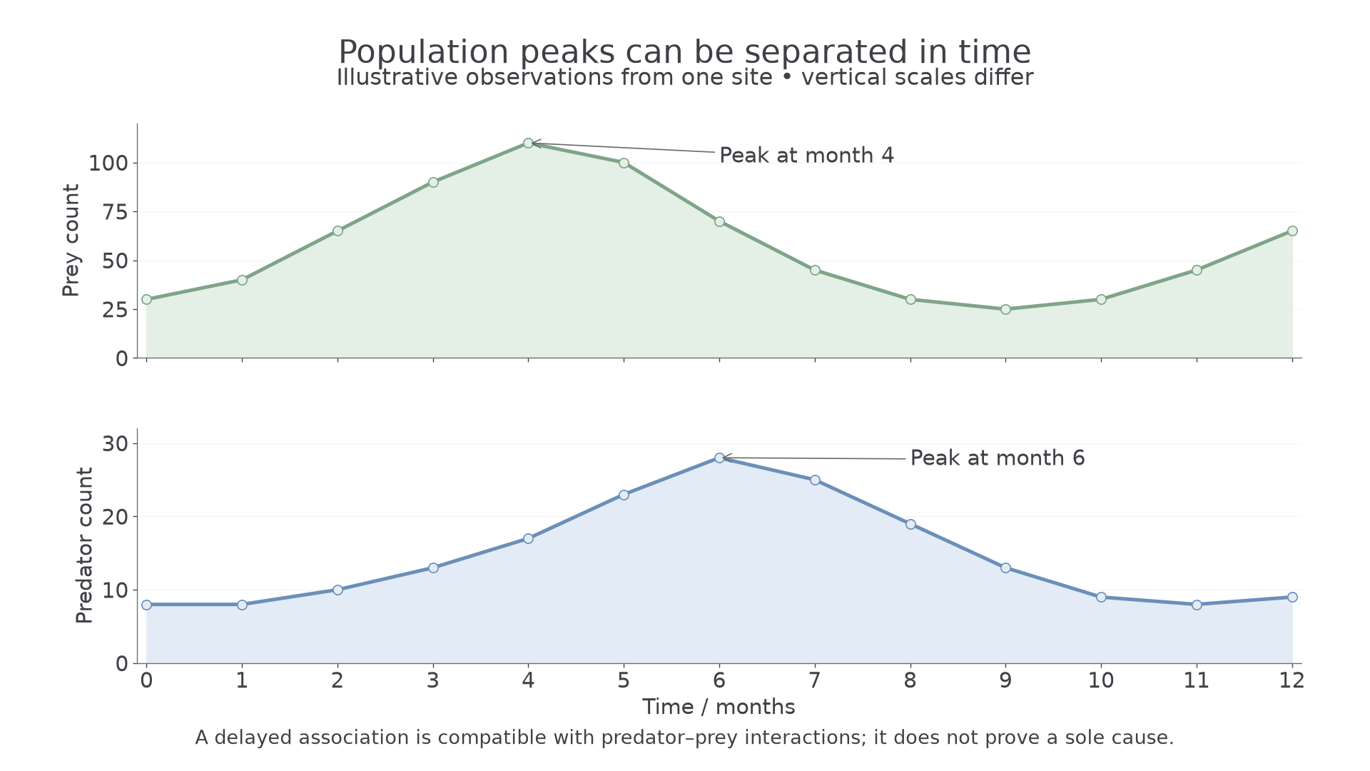
The prey peak comes first, which fits this cycle but does not prove it. Real populations also respond to weather, disease, immigration and alternative foods. Repeated years, other sites or diet evidence would test the explanation.

Estimating population size

You can rarely count every organism, so the sampling method depends on whether the organism moves.

Quadrats suit sessile (fixed in place) or slow-moving organisms; mark–release–recapture suits motile ones.

Random quadrats and belt transects

To estimate abundance across a whole area, place quadrats, frames of stated area, at random:

1. Map the site with perpendicular coordinate axes, such as two tapes.
2. Generate random coordinates, so that you do not choose promising patches by eye.
3. Place the same quadrat corner at each position. Do not throw quadrats.
4. Count using an agreed boundary rule for plants on the frame's edge.
5. Repeat in many quadrats, reducing the influence of chance patchiness, and calculate the mean.

A belt transect samples a strip across a gradient. Place quadrats continuously or at stated regular intervals along a tape, recording distance and abundance at each. This reveals distribution with distance. Repeated at independently chosen positions, transects can also estimate population size; a single one may be unrepresentative.

Density, frequency and cover

These describe different aspects of abundance:

• Density is number per unit area.
• Frequency is the proportion or percentage of sampled quadrats containing the species: one quadrat with 100 plants contributes one presence.
• Percentage cover estimates the proportion of ground occupied by a species' vertical projection: the area it covers when you look straight down from above. It is useful when individuals are hard to distinguish, as in grasses.

An unqualified "scale up" earned no mark in a 2024 question, so state the areas.

Mark–release–recapture

Motile organisms leave quadrats, so you estimate their number from how far a marked group is diluted:

1. Capture a first sample, mark individuals harmlessly and release them where caught.
2. Allow enough time for them to mix through the population.
3. Collect a second sample by a comparable method. Record its total size and the number marked.

The fraction marked in the second sample approximates the fraction marked in the whole population:

Using only the unmarked animals as $n_2$ gave a common wrong answer in a 2025 paper.

The estimate assumes the marked fraction stays representative:

• marks stay on, so recaptured animals are recognised
• marking does not affect survival or capture, for example by making animals easier for predators to see
• marked animals have time to mix through the population
• births, deaths, immigration and emigration are negligible between captures

Mark loss lowers observed $m$ and therefore tends to overestimate $N$. Trap-shy marked animals, or marks that make animals easier for predators to see, have the same effect, because fewer are recaptured. Sampling again before marked animals have mixed, close to where they were released, raises $m$ and so underestimates $N$.